The Central Limit Theorem: Laplace’s 1810 Memoir and Why the Long-Term Investor’s Friend Is Aggregation, Not Prediction

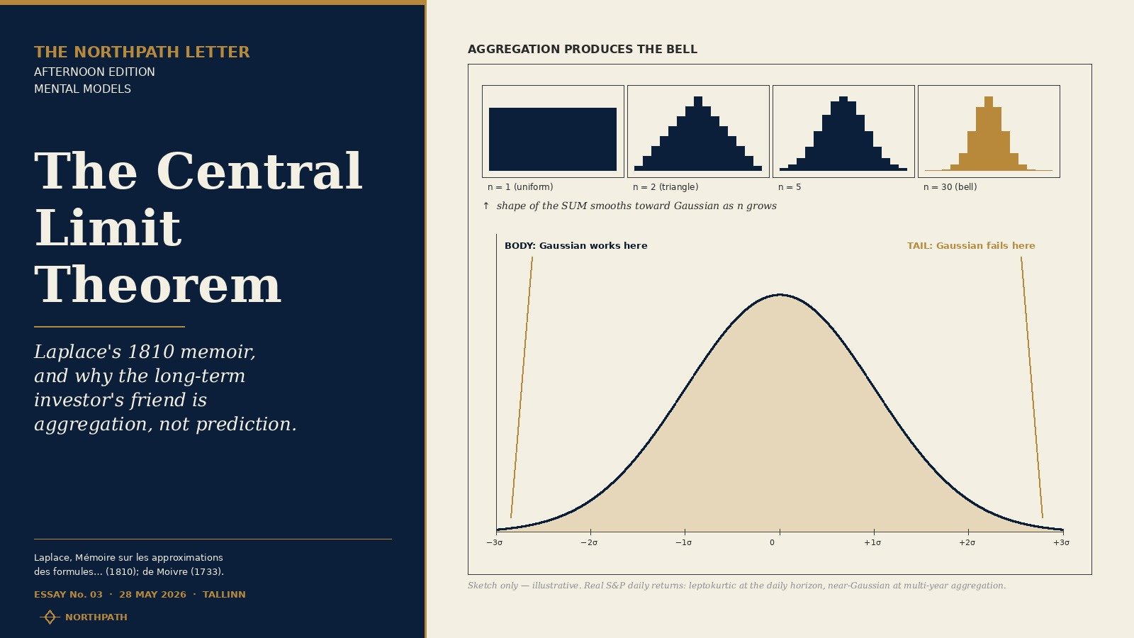
Editorial cover with bell curve and convergence histograms for the Central Limit Theorem essay

AFTERNOON EDITION — MENTAL MODELS · Essay No. 03 in the Mental Models series · The NorthPath Letter · 28 May 2026 · Tallinn

The Model — Laplace, 1810

The Central Limit Theorem is the most consequential theorem in probability theory for the long-term investor, and almost no investor knows its exact statement. In ordinary language it says: when you add up a large number of independent random influences, none of which is overwhelmingly large compared with the others, the distribution of the sum is approximately Gaussian — bell-shaped — no matter what the individual distributions look like. The bell curve is not a fact about nature. It is a fact about aggregation.

The first published general version appears in Pierre-Simon Laplace’s Mémoire sur les approximations des formules qui sont fonctions de très grands nombres et sur leur application aux probabilités, read to the Institut de France in April 1810 and printed in the Mémoires de l’Académie des Sciences later that year. Laplace generalised an earlier special case proved by Abraham de Moivre in The Doctrine of Chances (second edition, 1738; first stated in a 1733 supplement), in which de Moivre derived the bell-shaped approximation to the symmetric binomial. Stephen M. Stigler, in The History of Statistics: The Measurement of Uncertainty Before 1900 (Harvard, 1986, chapters 2 and 3), credits Laplace with extending the result to sums of independent variables drawn from arbitrary distributions and with embedding it in his programme of inverse probability. Lucien Le Cam’s monograph article “The Central Limit Theorem Around 1935” (Statistical Science, vol. 1, no. 1, 1986, pp. 78–96) traces the modern Lyapunov–Lindeberg–Feller rigorisation, which fixes both the conditions under which the theorem holds and, equally important, the conditions under which it fails.

The one-sentence form for an equity practitioner is this: the average of many small, independent, finite-variance shocks looks Gaussian even when each shock is not — and that fact is the entire architecture of risk management, factor models, Sharpe ratios, and modern portfolio theory. Strip the theorem away and almost every quantitative technique on a typical asset-management desk goes with it.

Convergence to Gaussian: distribution of sums of independent uniform variables for n=1, n=2, n=5, n=30, showing the bell curve emerging from aggregation
Figure 1. The Central Limit Theorem in action. The distribution of a single uniform draw is flat; sum two and it is a triangle; sum five and the bell shape is visible; sum thirty and the histogram is, for practical purposes, Gaussian. The shape of the individual contributors is irrelevant; the geometry of repeated convolution is the entire story.

The Mechanism

Why does aggregation produce a bell curve? Intuition first, formality second. Each random influence contributes some mean and some variance to the sum. When you add a great many of them, the means stack linearly but the variances also stack linearly — so the standard deviation of the sum grows only as the square root of n. The relative dispersion shrinks. What is left, once you standardise by that shrinking dispersion, is determined not by the shape of the individual contributors but by a deeper geometric fact about the convolution of probability densities. Convolution is a smoothing operation; repeated convolution drives the result toward the unique shape that is invariant under further convolution and standardisation. That fixed point is the Gaussian.

A more careful statement: if X₁, X₂, … are independent identically distributed random variables with finite mean μ and finite variance σ², then the standardised sum (X₁ + … + Xₙ − nμ) ⁄ (σ√n) converges in distribution to a standard normal as n grows without bound. The Lindeberg–Feller refinement weakens the identical-distribution assumption and replaces it with a condition that no single variable dominates the sum, formalised as the Lindeberg condition that the contribution of any individual term to the total variance must vanish in the limit.

Two things are essential and the long-term investor must internalise both. First: independence. The theorem says nothing about dependent variables that share a common shock. Second: finite variance. The theorem says nothing about variables drawn from distributions whose second moment does not exist. Both qualifications are central to what follows, and both are violated routinely in the financial world.

The Empirical Record

Equity returns over short horizons emphatically do not follow a normal distribution. The classic stylised facts, catalogued by Rama Cont in “Empirical Properties of Asset Returns: Stylized Facts and Statistical Issues” (Quantitative Finance, vol. 1, no. 2, 2001, pp. 223–236), are: heavy tails — excess kurtosis of daily returns is routinely above ten — volatility clustering, leverage effects, and what Cont labels “aggregational Gaussianity,” the empirical observation that the distribution looks more bell-shaped at monthly and quarterly horizons than at daily horizons. The Central Limit Theorem does operate on equity returns, but slowly, and only because daily returns are neither truly independent nor drawn from a stationary distribution.

Eugene F. Fama’s 1965 PhD work, “The Behavior of Stock Market Prices” (Journal of Business, vol. 38, no. 1, pp. 34–105), found that daily stock returns are leptokurtic and rejected the simple Gaussian model. Benoit Mandelbrot’s earlier “The Variation of Certain Speculative Prices” (Journal of Business, vol. 36, no. 4, 1963, pp. 394–419) had already proposed stable Paretian distributions with infinite variance — distributions to which the classical CLT does not apply. The empirical picture six decades on is that the Gaussian arrives at aggregation horizons measured in months and years, not days, and even then only as an approximation that breaks down in the tails.

The Bank for International Settlements Quarterly Review of December 2019 noted that the September 2019 US repo-market spike, which a standard one-factor Gaussian model would have placed at roughly a 1-in-10⁹ probability, had in fact occurred within ten years of the previous comparable dislocation. The US Office of Financial Research’s Annual Report (2020) made the same point for equities: the 12 March 2020 single-day −9.5% S&P 500 close was, under a Gaussian volatility regime calibrated to the prior year, a roughly 10-sigma event — once in many billions of years on a Gaussian planet. We are not on a Gaussian planet at the daily frequency, but we drift toward one as the aggregation window widens.

The European Securities and Markets Authority’s annual Trends, Risks and Vulnerabilities Report (2024 edition) reaches a complementary conclusion from the regulator’s perspective. Across the 2015–2023 period, single-day European blue-chip equity moves of greater than four standard deviations occurred roughly nine times more often than a constant-volatility Gaussian model would predict, and the excess was concentrated in clustered episodes — March 2020, September 2022, March 2023 — that violated independence within the cluster while otherwise looking benign. The supervisor’s operational conclusion is the one a thoughtful investor should already have reached: the Gaussian framework is a useful default for setting capital under normal conditions, and a dangerously misleading default for setting capital under stress conditions.

Bar chart comparing empirical S&P 500 daily return distribution to fitted Gaussian: body fits closely, tails diverge by orders of magnitude beyond ±4σ
Figure 2. The empirical CLT verdict on equity returns. Stylised representation of S&P 500 daily return frequencies versus the best-fit Gaussian on a log frequency scale. The body of the empirical distribution tracks the bell curve. The tails diverge by orders of magnitude. The lesson for the operator: trust the bell in the middle, distrust it at the edge.

Two Historical Episodes

The collapse of Long-Term Capital Management in September 1998 is the textbook study of misapplied CLT. Roger Lowenstein’s When Genius Failed: The Rise and Fall of Long-Term Capital Management (Random House, 2000) and the President’s Working Group on Financial Markets report “Hedge Funds, Leverage, and the Lessons of Long-Term Capital Management” (April 1999) document the firm’s value-at-risk machinery, which assumed that daily P&L was approximately Gaussian with variance estimated from a rolling five-year window. Convergence trades — long off-the-run US Treasuries against short on-the-run; long Italian government bonds against short German Bunds; equity-pair arbitrages — were sized so that a one-day standard deviation of book P&L was roughly forty-five million dollars on equity of four-and-three-quarter billion. The model implied that a one-billion-dollar daily loss carried a probability of approximately one in 10²⁴. The fund lost five hundred and fifty-three million dollars on a single day, 21 August 1998, and was insolvent within five weeks. The independence assumption had failed: when the Russian sovereign default touched off a global flight to liquidity, every supposedly independent trade became one and the same bet on the willingness of leveraged intermediaries to provide funding.

The 19 October 1987 crash is the older episode. The Dow Jones Industrial Average fell 22.6% in a single trading session. Under the lognormal model that underpinned the Black–Scholes pricing of the portfolio-insurance strategies that contributed to the cascade, a one-day move of that magnitude was a roughly 20-sigma event — frequency-equivalent to once in many times the age of the universe. The Brady Commission’s Report of the Presidential Task Force on Market Mechanisms (January 1988) attributed the cascade to feedback among index futures, programme trading, and portfolio insurance — three features that violated the independence assumption simultaneously. Mark Rubinstein, one of the architects of the insurance approach, later acknowledged in his Frank J. Fabozzi Memorial Lecture (2000) that the model had treated the insurance-driven order flow as exogenous when in fact, at scale, it was the dominant endogenous shock. The operational point is that risk frameworks built on the CLT manufactured a false sense of safety in regimes where independence was the first thing to break.

Application to Long-Term Equity Investing — Three Operating Disciplines

The first discipline is to know whether you are in CLT territory before you trust an average. Aggregation across many independent positions, holding periods, or business cycles is the equity investor’s friend. Aggregation across positions that share a common factor is a false friend. A portfolio of fifty mid-cap equities held for twenty years across multiple credit and policy cycles has many of the independence properties the CLT requires. A portfolio of fifty European peripheral-sovereign-exposed banks held over a quarter does not, because every name in it is a single, repeated bet on one shared variable. The first practical test before relying on a portfolio-level Sharpe ratio or standard deviation is to ask: in the bad case, do these positions move together?

The second discipline is to keep finite variance on your side. Variance is finite when the worst possible single outcome is bounded — when individual position size is capped, when leverage is bounded, when any single illiquid concentrated bet does not exceed a defined fraction of capital. Variance becomes effectively infinite the moment a single trade can wipe out the book. This is the operational meaning of Munger’s “rule of intelligent compounding”: survive each year, and the CLT will reward you over decades. It is also the meaning of Buffett’s two rules about not losing money: a single ruinous draw turns the iterated multiplication of returns from a long-run Gaussian-in-logarithms into a zero, and the theorem cannot save a series whose product has been multiplied by nought.

The third discipline is to distrust the bell curve in the tail and trust it in the body. The mid-distribution behaviour of well-diversified equity portfolios at multi-year horizons is genuinely close to Gaussian, and Sharpe ratios, mean-variance optimisation, and standard deviation are useful descriptive tools there. In the tail — drawdowns of thirty per cent, forty per cent, fifty per cent — the Gaussian model understates frequency by orders of magnitude. The long-term investor uses the bell curve for the body of the distribution to set position sizes and to evaluate strategies, and uses non-Gaussian thinking — scenario analysis, stress testing, leverage limits, liquidity buffers, written-down pre-mortems — for the tail.

Three-card framework: discipline 1 manage independence, discipline 2 cap variance, discipline 3 separate body from tail
Figure 3. Three operating disciplines that translate the Central Limit Theorem into an equity operating manual. Manage independence so the n in √n is real; cap variance so the theorem’s preconditions hold; split the bell curve into a body framework and a tail framework, and refuse to use one tool for the other.

How the Long-Term Equity Tradition Has Used It

Warren Buffett has been disarming about distributional assumptions. In the Berkshire Hathaway 1993 chairman’s letter, discussing the use of beta and standard deviation as proxies for risk, he wrote that academic definitions of risk wander off into absurdity once they require treating market volatility as the relevant measure for a long-term owner of a business. The implicit critique is that the Gaussian framework is the right tool for some questions — portfolio-level dispersion over many independent owners and many quarters — and the wrong tool for others, notably the probability of permanent loss of capital on a single concentrated position. The 2002 letter, in the famous passage on derivatives as “financial weapons of mass destruction,” sharpens the same point: when independence breaks, the standard deviation of P&L is no longer a meaningful summary statistic, because the joint distribution has collapsed to a single shared move.

Howard Marks’s Oaktree memo “Risk” (January 2006), later reprinted as a chapter in The Most Important Thing (Columbia University Press, 2011), takes the same view from the tail-of-the-distribution side. Marks argues that risk is the probability of an unacceptable outcome, not the dispersion of outcomes — a definition that is dual to the CLT. His later memo “Investing Without People” (June 2018) returns to the idea in the context of passive-vehicle flows: as more capital is allocated to vehicles that trade in lockstep, the independence assumption underlying any portfolio-diversification benefit shrinks, and the effective n in the √n denominator of the CLT collapses.

Charlie Munger’s “A Lesson on Elementary, Worldly Wisdom as It Relates to Investment Management and Business,” delivered at the USC Marshall School in April 1994 and reprinted in Poor Charlie’s Almanack (Donning, 2005), makes the most economical case for why the long-term investor must understand the CLT. Munger argues that compounding — the long-term equity investor’s central mechanism — is intelligible only as the iterated multiplication of independent returns, and that the geometric structure of the result is, in logarithms, essentially Gaussian. The discipline is to keep the inputs roughly independent, keep their variance bounded, and let arithmetic do the rest.

Nick Sleep’s Nomad Investment Partnership letters (2001 to 2014, collected and reprinted in Nomad Investment Partnership Letters to Partners, 2021) repeatedly invoke aggregation logic: fewer decisions, smaller variance per decision, more time for compounding. Sleep’s portfolio concentration is unusual, but the principle — keep the number of large independent bets finite and well-understood — is a deliberate refusal to be ambushed by the failure modes of large-n CLT thinking, which silently assumes a great many small bets are genuinely independent when in fact they are correlated through factor exposure. François Rochon’s Giverny Capital quarterly letters, archived on the firm’s website since 1998, make the same observation about diversification from the other direction: beyond roughly twenty-five well-understood positions, the marginal CLT benefit is exhausted, and additional names dilute analytical attention without reducing systematic variance.

Key Takeaways

The Central Limit Theorem is not a description of nature. It is a description of what happens when you average independent, finite-variance random variables. The two assumptions — independence and finite variance — are the entirety of the engineering safety question for any portfolio that treats Gaussian statistics as its working language.

Equity returns approach Gaussian shape only at long aggregation horizons and only in the body of the distribution. The tails remain heavier than the bell curve for as long as anyone has measured them, and the documented stylised fact of aggregational Gaussianity is exactly that — an approach, not an arrival.

The CLT explains why broad, long-duration index investing tends to look close to its model, and why concentrated, short-duration, leveraged trading tends not to. The investor who builds one operating system around the CLT’s body and a separate operating system around its tail is treating the theorem honestly. The investor who applies the body’s tools to the tail will, sooner or later, blow up.

Two of the most studied failures of CLT-based risk management — Long-Term Capital Management in 1998 and the 1987 crash — both stemmed from violating the independence assumption, not from any defect in the theorem itself. Independence is the assumption that breaks first in a panic, because a panic is by definition the moment when one common factor swamps every supposedly idiosyncratic shock.

The long-term equity tradition — Buffett, Munger, Marks, Sleep, Rochon — has converged on a simple operating discipline that is the CLT made human: keep position sizes bounded so variance stays finite, keep correlations honest so independence stays approximately true, and let aggregation across many years do the work the theorem promises.

— Manish Goel, FCA / NorthPath Advisory OÜ / Tallinn, Estonia

Important.
All content on this site and in this email is journalism and education for a general audience. Nothing here constitutes investment advice or a recommendation in respect of any specific financial instrument, nor an offer or solicitation to buy or sell any security. Readers should consult an authorised financial adviser regulated in their own jurisdiction before making any investment decision.