Category: Mental Models

AFTERNOON EDITION — Mental Models

In the summer of 1885, Francis Galton stood before the Royal Anthropological Institute in London with a curious finding. He had measured the heights of 928 adult children and 205 of their parents, and noticed that the offspring of unusually tall parents tended to be tall — but less tall than the parents. The offspring of unusually short parents tended to be short — but less short. Each generation, in other words, drifted back toward the average of the population. He published the lecture the following year in the Institute’s Journal under a title he chose with care: “Regression towards Mediocrity in Hereditary Stature.”

For Galton, the word “mediocrity” was statistical, not pejorative. He had stumbled on the first mathematical description of a phenomenon that now sits under nearly every empirical exercise in finance, medicine, sports, education, and public policy: when a measurement is the sum of a stable component and a noisy one, an extreme observation in the first period will be followed, on average, by a less extreme observation in the second. The drift is not punishment for excellence. It is the arithmetic of noise.

1. The model — Galton 1886, in his own words

The canonical citation is Francis Galton, “Regression towards Mediocrity in Hereditary Stature,” Journal of the Anthropological Institute of Great Britain and Ireland, vol. 15 (1886), pp. 246–263. Galton’s own one-sentence form, set out on page 252, is the cleanest definition we have: the deviation of the offspring from the population average is, on average, two-thirds of the corresponding deviation of the parents. He called that coefficient — the two-thirds — the “ratio of regression.” When modern statisticians later rebadged the linear technique he had invented as “regression analysis,” they preserved his accidental terminology long after the population-genetics origin had faded.

A stricter contemporary form, due to Karl Pearson’s 1903 generalisation in Biometrika, runs as follows. If X and Y are correlated with coefficient r, and both are standardised to zero mean and unit variance, then the conditional expectation of Y given X is exactly r · X. Whenever the absolute value of r is less than one — which is to say, whenever the two variables are not perfectly correlated — the predicted Y is closer to its mean than X was to its own. The mean is the gravitational centre toward which any less-than-perfectly-correlated system is pulled.

Galton’s discovery survives one essential restatement for the modern reader: the phenomenon does not require any causal mechanism. It is a property of measurement under uncertainty. Stephen Stigler, the historian of statistics, has written that this is the single most under-taught idea in quantitative reasoning, precisely because it produces effects that the naïve mind insistently re-narrates as cause and effect (Stigler, Statistics on the Table, Harvard University Press, 1999, chapter 9). The investor who internalises only one rule from this essay should internalise that one: when an extreme draws an explanation, the explanation may simply be the arithmetic.

2. The mechanism — why the drift is unavoidable

The cleanest way to see why regression must happen is to decompose any observed outcome into two parts: a persistent component, call it Skill, and a transient component, call it Luck. Suppose we observe the top decile of a population — top-decile mutual-fund managers, top-decile athletes, top-decile parental heights. By definition, these observations carry unusually favourable Luck draws on top of whatever Skill they possess. In the next period, Skill persists by assumption, but Luck — being the noisy component — is, by definition, drawn afresh from a distribution centred on zero. The expected new observation is therefore Skill plus zero, lower than Skill plus favourable Luck. The top decile must, on average, fall back toward the mean.

The size of the drift is governed by one ratio: the share of total variance contributed by Skill. If a domain is mostly Skill — Olympic sprint times for elite athletes after years of selection — regression will be small. If it is mostly Luck — single-quarter mutual-fund returns — regression will be enormous. Michael Mauboussin’s 2012 book The Success Equation (Harvard Business Review Press) titled this the “skill-luck continuum” and made the point that the investor’s first job in nearly every empirical domain is to estimate that ratio before extrapolating a single number.

It follows that regression is asymmetric in a useful way. Extreme outcomes regress most strongly. Performance near the mean barely regresses at all. The investor who learns to feel the pull harder at the tails — both the celebrated top and the punished bottom — is doing the work of the model. And it follows, too, that the drift is on the conditional expectation: there is no guarantee that any specific top-decile observation will fall back, only that the average of all top-decile observations will. The mistake of applying a population property to one individual is the ecological fallacy in reverse, and it is endemic in financial commentary.

3. The empirical record — three exhibits from active equity

The financial evidence on mean reversion is, on the whole, embarrassingly consistent. Three exhibits.

Mark Carhart’s 1997 paper “On Persistence in Mutual Fund Performance” (Journal of Finance 52(1): 57–82) examined the entire universe of US diversified equity funds from 1962 to 1993, sorted them into deciles each year on the basis of their previous-year return, and tracked the next-year performance. After adjusting for the market, size, value, and momentum factors he had assembled, the persistence of top-decile alpha was statistically indistinguishable from zero. The bottom decile, by contrast, persisted — bad funds stayed bad, largely because of expenses and turnover. The implication is the one Galton would have predicted: the favoured deciles are dominated by noise, and noise regresses; the disfavoured deciles include a structural deadweight (fees) that does not.

S&P Dow Jones Indices has run a quarterly persistence scorecard for two decades. In the U.S. Persistence Scorecard Year-End 2024, the share of top-quartile US large-cap funds that remained top-quartile across the next five calendar years was 0%. That is not a misprint. Reading the same scorecard for the mid-2025 update, only 29% of top-quartile large-cap funds maintained their position even over a subsequent two-year window. A coin flip would have predicted 25% over two years and roughly 0.4% over five. Active equity performance is now indistinguishable, in persistence terms, from random selection followed by regression. The mathematics permits a sharper statement: the noisier the signal you select on, the less of it survives the second draw.

The corporate analogue is no less stark. Robert Wiggins and Timothy Ruefli, in “Sustained Competitive Advantage: Temporal Dynamics and the Incidence and Persistence of Superior Economic Performance” (Organization Science 13(1), 2002: 81–105), studied the return on assets of 6,772 firms across 40 industries between 1972 and 1997. Of the firms that achieved “superior” returns in their stratum, only about 5% sustained that position for 10 years or more, and just 0.5% for 20 years. The default destination of an above-average return-on-assets number is the industry mean, and the rate of decay can be calibrated. McKinsey’s repeat of the exercise in Valuation (Koller, Goedhart and Wessels, 7th edition, 2020, chapter 8) finds the same shape: the median high-ROIC firm gives back about half its excess return within seven to ten years.

4. Two historical episodes

Israeli flight school, 1969. Daniel Kahneman, then a young consulting psychologist for the Israeli Air Force, was lecturing senior flight instructors on the established behavioural finding that praise produces better learning outcomes than punishment. A grizzled instructor objected. With respect, sir, he said in effect, what you are saying is for the birds: I have many times praised flight cadets for the clean execution of some aerobatic manoeuvre, and the next time they tried it they did worse; I have often screamed into a cadet’s earphone for bad execution and on the next try he improved. Kahneman writes that the moment was the most important insight of his early career. The cadets’ performance was a noisy signal around a stable mean. A spectacularly clean manoeuvre was, by definition, mostly luck on top of skill; the next attempt would regress whether the instructor praised or screamed. The instructor had been the unwitting witness to thirty years of regression to the mean, mistaking statistical gravity for causation. The episode is recounted in Kahneman, Thinking, Fast and Slow (Farrar, Straus and Giroux, 2011), chapter 17, and its formal version had appeared four decades earlier in Kahneman and Tversky, “On the Psychology of Prediction,” Psychological Review 80(4), 1973: 237–251.

Sports Illustrated cover jinx. From 1954 onward the legend within the magazine was that any athlete or team gracing the cover would subsequently underperform. In a 2002 internal review the editors counted 913 covers; 37% had been followed by some “decline.” Statisticians who examined the data — including Schaffer (2002) and Smith and Smith (2011) — found no jinx at all, only the regression Galton had described 116 years earlier. Cover athletes were, almost by selection, drawn from the upper tail of recent performance; mean reversion guaranteed that the next month would be statistically less impressive than the month that had earned them the cover. The “jinx” was a narrative built around the arithmetic of selection.

Both episodes carry the same warning for the investor: when an observation is selected because it is extreme, the next observation will, on average, be less extreme. Any narrative that explains the change in causal terms — the cover cursed him, the praise spoiled her, the new CEO destroyed the franchise — is a narrative that may simply be re-describing regression. The mind reaches for a story; the spreadsheet would have suggested gravity.

5. Application to long-term equity investing

Three operating disciplines fall directly out of Galton’s mathematics.

Discipline one: never project the past five years of profit margins straight into the future. The single most reliable mean-reverting series in financial history is the corporate profit share of national income — what GMO’s Jeremy Grantham has called, only half-joking, the most mean-reverting series in finance. The mechanism is the one Adam Smith identified in The Wealth of Nations (1776, Book I, Chapter VII): high margins attract competition, low margins repel it. The empirical record in the United States, where post-1947 National Income and Product Accounts data permits a long view, shows after-tax corporate profit margins oscillating in a relatively narrow band around 6 to 8 percent of GDP, with each excursion to either extreme corrected within roughly a decade. A discounted-cash-flow model that capitalises peak margins as a terminal-year assumption will, in regression-to-the-mean terms, systematically overstate intrinsic value at cycle peaks and understate it at troughs. The corrective is mechanical: stress-test every long-duration model with a margin path that reverts to a sector mean within ten years, and require the investment thesis to survive that test.

Discipline two: when selecting active managers — including selecting oneself as one’s own active manager — discount the persistence of recent outperformance to roughly nil after five years. The Carhart finding, replicated in every multi-year SPIVA scorecard, is that top-decile performance over one-, three-, and five-year windows is almost entirely a noise phenomenon, with one important exception: costs and structural disadvantages — high fees, poor execution, persistent leverage at the wrong points in the cycle — produce real persistence on the downside. The investor’s manager-selection model should therefore be asymmetric. Be sceptical of celebrated past returns; take negative persistence seriously as a structural signal rather than a temporary embarrassment.

Discipline three: at extremes of valuation, the price-multiple itself becomes the dominant mean-reverting variable. Robert Shiller’s cyclically adjusted price-earnings ratio (CAPE), constructed in Campbell and Shiller, “Stock Prices, Earnings, and Expected Dividends,” Journal of Finance 43 (1988), has the unhappy distinction of explaining roughly 40 percent of the variance in subsequent ten-year real US equity returns since 1881. The mechanism is again Galton’s: peak multiples, like peak margins, are by definition the joint product of fundamentals and noise, and the noisy component regresses. This is not a market-timing claim — short-horizon predictability is essentially zero — but a discipline against starting positions at extreme starting multiples without a compensating margin of safety. The investor who buys at the 95th percentile of CAPE and waits ten years must expect that the median outcome will be set largely by multiple compression, not by underlying earnings growth.

6. How the long-term equity tradition has used it

Howard Marks, in his July 2003 memo “The Most Important Thing” and the May 2001 memo “You Can’t Predict, You Can Prepare,” made regression to the mean the engine of his cycle theory. The Oaktree pendulum, Marks wrote, swings not from euphoria to despair because anyone wills it to, but because the very behaviours that produce extreme valuations contain the seeds of their reversal: high valuations attract supply of paper and erode prospective returns until the marginal buyer rebels; low valuations starve supply and improve prospective returns until the marginal seller capitulates. In his 2011 book of the same name, The Most Important Thing: Uncommon Sense for the Thoughtful Investor (Columbia Business School Publishing, 2011), Marks devotes an entire chapter — chapter 8, “Being Attentive to Cycles” — to the proposition that the investor who fails to internalise mean reversion will be most aggressive when prospective returns are lowest and most defensive when they are highest. His operating heuristic, articulated again in the September 2014 memo “Risk Revisited,” is to scale risk-taking inversely with prevailing valuations, precisely because of the Galton mechanism.

Jeremy Grantham at GMO has built the firm’s seven-year asset-class forecast on the same idea. In a sequence of quarterly letters from 1994 onward, and in the February 2012 letter “The Longest Quarterly Letter Ever,” Grantham observes that profit margins and price-earnings ratios are the two great mean-reverting variables in equity markets, and that GMO’s forecasts assume both will return to their long-run averages within seven years. His June 2017 piece, “This Time Seems Very, Very Different,” extended the framework with a candid admission: in the platform-monopoly era, the speed of regression in margins has slowed; he now models a fifteen-to-twenty-year half-life for profit-share reversion rather than the seven years that prevailed from 1900 to 1997. The model survives; only the time constant has changed. The GMO seven-year forecast remains the most public mean-reversion betting card in the industry, and its track record — broadly accurate on direction across decadal windows, frequently early on timing — is precisely what one would expect from a model that uses Galton’s gravity correctly but cannot pin the exact moment of return.

Warren Buffett, characteristically, has acknowledged the same gravity while resisting its full implications for the highest-quality franchises. In his 1989 Berkshire Hathaway letter (“Mistakes of the First 25 Years”) he wrote that he had repeatedly paid too little attention to the tendency of high returns on capital to attract competition, and too much attention to apparently cheap statistical bargains where the underlying economics were quietly regressing toward unprofitability. His later doctrine — pay a fair price for a wonderful business — is in part an acknowledgement that some businesses, by virtue of structural moats, regress more slowly than the average, but not that they regress not at all. The 1999 Sun Valley speech, reprinted in Fortune on 22 November 1999 under the title “Mr. Buffett on the Stock Market,” is a sustained warning that aggregate US after-tax corporate profits have been mean-reverting against GDP for the entire post-war period and will not, contrary to the late-1990s consensus, settle permanently at a higher plateau.

The discipline these three practitioners share is not market timing but probability-weighting. Each builds his portfolio around the prior that extreme observations — of returns, of margins, of multiples — will, on average, fall back toward a mean that one can estimate from a long enough history. The variance of each individual outcome remains large; the directionality of the conditional expectation does not.

7. Key takeaways

Galton’s regression is a property of measurement under uncertainty, not a causal force; the mind insists on re-narrating it as one and the investor must resist that re-narration. The strength of the pull is set by the ratio of Skill variance to Luck variance, and that ratio must be estimated domain by domain before extrapolating any extreme observation. In equity markets, the two great mean-reverting variables are profit margins and valuation multiples, and every long-duration model should be stress-tested with a path that reverts both within ten to fifteen years. Manager-selection should be asymmetric: discount celebrated outperformance toward random, but take poor performance and high costs as the persistent signals they are. In cycle terms, the Oaktree pendulum and the GMO forecast both encode the same Galton insight; the investor who internalises it tends, over decades, to take risk when others will not and to take risk off when others crowd in. The model is 140 years old; its tax on the investor who ignores it is paid afresh in every cycle.

— Manish Goel, FCA / NorthPath Advisory OÜ / Tallinn, Estonia

Important. All content on this site and in this email is journalism and education for a general audience. Nothing here constitutes investment advice or a recommendation in respect of any specific financial instrument, nor an offer or solicitation to buy or sell any security. Readers should consult an authorised financial adviser regulated in their own jurisdiction before making any investment decision.

AFTERNOON EDITION — MENTAL MODELS · Essay No. 03 in the Mental Models series · The NorthPath Letter · 28 May 2026 · Tallinn

The Model — Laplace, 1810

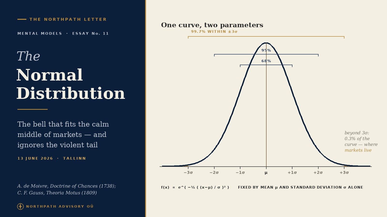
The Central Limit Theorem is the most consequential theorem in probability theory for the long-term investor, and almost no investor knows its exact statement. In ordinary language it says: when you add up a large number of independent random influences, none of which is overwhelmingly large compared with the others, the distribution of the sum is approximately Gaussian — bell-shaped — no matter what the individual distributions look like. The bell curve is not a fact about nature. It is a fact about aggregation.

The first published general version appears in Pierre-Simon Laplace’s Mémoire sur les approximations des formules qui sont fonctions de très grands nombres et sur leur application aux probabilités, read to the Institut de France in April 1810 and printed in the Mémoires de l’Académie des Sciences later that year. Laplace generalised an earlier special case proved by Abraham de Moivre in The Doctrine of Chances (second edition, 1738; first stated in a 1733 supplement), in which de Moivre derived the bell-shaped approximation to the symmetric binomial. Stephen M. Stigler, in The History of Statistics: The Measurement of Uncertainty Before 1900 (Harvard, 1986, chapters 2 and 3), credits Laplace with extending the result to sums of independent variables drawn from arbitrary distributions and with embedding it in his programme of inverse probability. Lucien Le Cam’s monograph article “The Central Limit Theorem Around 1935” (Statistical Science, vol. 1, no. 1, 1986, pp. 78–96) traces the modern Lyapunov–Lindeberg–Feller rigorisation, which fixes both the conditions under which the theorem holds and, equally important, the conditions under which it fails.

The one-sentence form for an equity practitioner is this: the average of many small, independent, finite-variance shocks looks Gaussian even when each shock is not — and that fact is the entire architecture of risk management, factor models, Sharpe ratios, and modern portfolio theory. Strip the theorem away and almost every quantitative technique on a typical asset-management desk goes with it.

The Mechanism

Why does aggregation produce a bell curve? Intuition first, formality second. Each random influence contributes some mean and some variance to the sum. When you add a great many of them, the means stack linearly but the variances also stack linearly — so the standard deviation of the sum grows only as the square root of n. The relative dispersion shrinks. What is left, once you standardise by that shrinking dispersion, is determined not by the shape of the individual contributors but by a deeper geometric fact about the convolution of probability densities. Convolution is a smoothing operation; repeated convolution drives the result toward the unique shape that is invariant under further convolution and standardisation. That fixed point is the Gaussian.

A more careful statement: if X₁, X₂, … are independent identically distributed random variables with finite mean μ and finite variance σ², then the standardised sum (X₁ + … + Xₙ − nμ) ⁄ (σ√n) converges in distribution to a standard normal as n grows without bound. The Lindeberg–Feller refinement weakens the identical-distribution assumption and replaces it with a condition that no single variable dominates the sum, formalised as the Lindeberg condition that the contribution of any individual term to the total variance must vanish in the limit.

Two things are essential and the long-term investor must internalise both. First: independence. The theorem says nothing about dependent variables that share a common shock. Second: finite variance. The theorem says nothing about variables drawn from distributions whose second moment does not exist. Both qualifications are central to what follows, and both are violated routinely in the financial world.

The Empirical Record

Equity returns over short horizons emphatically do not follow a normal distribution. The classic stylised facts, catalogued by Rama Cont in “Empirical Properties of Asset Returns: Stylized Facts and Statistical Issues” (Quantitative Finance, vol. 1, no. 2, 2001, pp. 223–236), are: heavy tails — excess kurtosis of daily returns is routinely above ten — volatility clustering, leverage effects, and what Cont labels “aggregational Gaussianity,” the empirical observation that the distribution looks more bell-shaped at monthly and quarterly horizons than at daily horizons. The Central Limit Theorem does operate on equity returns, but slowly, and only because daily returns are neither truly independent nor drawn from a stationary distribution.

Eugene F. Fama’s 1965 PhD work, “The Behavior of Stock Market Prices” (Journal of Business, vol. 38, no. 1, pp. 34–105), found that daily stock returns are leptokurtic and rejected the simple Gaussian model. Benoit Mandelbrot’s earlier “The Variation of Certain Speculative Prices” (Journal of Business, vol. 36, no. 4, 1963, pp. 394–419) had already proposed stable Paretian distributions with infinite variance — distributions to which the classical CLT does not apply. The empirical picture six decades on is that the Gaussian arrives at aggregation horizons measured in months and years, not days, and even then only as an approximation that breaks down in the tails.

The Bank for International Settlements Quarterly Review of December 2019 noted that the September 2019 US repo-market spike, which a standard one-factor Gaussian model would have placed at roughly a 1-in-10⁹ probability, had in fact occurred within ten years of the previous comparable dislocation. The US Office of Financial Research’s Annual Report (2020) made the same point for equities: the 12 March 2020 single-day −9.5% S&P 500 close was, under a Gaussian volatility regime calibrated to the prior year, a roughly 10-sigma event — once in many billions of years on a Gaussian planet. We are not on a Gaussian planet at the daily frequency, but we drift toward one as the aggregation window widens.

The European Securities and Markets Authority’s annual Trends, Risks and Vulnerabilities Report (2024 edition) reaches a complementary conclusion from the regulator’s perspective. Across the 2015–2023 period, single-day European blue-chip equity moves of greater than four standard deviations occurred roughly nine times more often than a constant-volatility Gaussian model would predict, and the excess was concentrated in clustered episodes — March 2020, September 2022, March 2023 — that violated independence within the cluster while otherwise looking benign. The supervisor’s operational conclusion is the one a thoughtful investor should already have reached: the Gaussian framework is a useful default for setting capital under normal conditions, and a dangerously misleading default for setting capital under stress conditions.

Two Historical Episodes

The collapse of Long-Term Capital Management in September 1998 is the textbook study of misapplied CLT. Roger Lowenstein’s When Genius Failed: The Rise and Fall of Long-Term Capital Management (Random House, 2000) and the President’s Working Group on Financial Markets report “Hedge Funds, Leverage, and the Lessons of Long-Term Capital Management” (April 1999) document the firm’s value-at-risk machinery, which assumed that daily P&L was approximately Gaussian with variance estimated from a rolling five-year window. Convergence trades — long off-the-run US Treasuries against short on-the-run; long Italian government bonds against short German Bunds; equity-pair arbitrages — were sized so that a one-day standard deviation of book P&L was roughly forty-five million dollars on equity of four-and-three-quarter billion. The model implied that a one-billion-dollar daily loss carried a probability of approximately one in 10²⁴. The fund lost five hundred and fifty-three million dollars on a single day, 21 August 1998, and was insolvent within five weeks. The independence assumption had failed: when the Russian sovereign default touched off a global flight to liquidity, every supposedly independent trade became one and the same bet on the willingness of leveraged intermediaries to provide funding.

The 19 October 1987 crash is the older episode. The Dow Jones Industrial Average fell 22.6% in a single trading session. Under the lognormal model that underpinned the Black–Scholes pricing of the portfolio-insurance strategies that contributed to the cascade, a one-day move of that magnitude was a roughly 20-sigma event — frequency-equivalent to once in many times the age of the universe. The Brady Commission’s Report of the Presidential Task Force on Market Mechanisms (January 1988) attributed the cascade to feedback among index futures, programme trading, and portfolio insurance — three features that violated the independence assumption simultaneously. Mark Rubinstein, one of the architects of the insurance approach, later acknowledged in his Frank J. Fabozzi Memorial Lecture (2000) that the model had treated the insurance-driven order flow as exogenous when in fact, at scale, it was the dominant endogenous shock. The operational point is that risk frameworks built on the CLT manufactured a false sense of safety in regimes where independence was the first thing to break.

Application to Long-Term Equity Investing — Three Operating Disciplines

The first discipline is to know whether you are in CLT territory before you trust an average. Aggregation across many independent positions, holding periods, or business cycles is the equity investor’s friend. Aggregation across positions that share a common factor is a false friend. A portfolio of fifty mid-cap equities held for twenty years across multiple credit and policy cycles has many of the independence properties the CLT requires. A portfolio of fifty European peripheral-sovereign-exposed banks held over a quarter does not, because every name in it is a single, repeated bet on one shared variable. The first practical test before relying on a portfolio-level Sharpe ratio or standard deviation is to ask: in the bad case, do these positions move together?

The second discipline is to keep finite variance on your side. Variance is finite when the worst possible single outcome is bounded — when individual position size is capped, when leverage is bounded, when any single illiquid concentrated bet does not exceed a defined fraction of capital. Variance becomes effectively infinite the moment a single trade can wipe out the book. This is the operational meaning of Munger’s “rule of intelligent compounding”: survive each year, and the CLT will reward you over decades. It is also the meaning of Buffett’s two rules about not losing money: a single ruinous draw turns the iterated multiplication of returns from a long-run Gaussian-in-logarithms into a zero, and the theorem cannot save a series whose product has been multiplied by nought.

The third discipline is to distrust the bell curve in the tail and trust it in the body. The mid-distribution behaviour of well-diversified equity portfolios at multi-year horizons is genuinely close to Gaussian, and Sharpe ratios, mean-variance optimisation, and standard deviation are useful descriptive tools there. In the tail — drawdowns of thirty per cent, forty per cent, fifty per cent — the Gaussian model understates frequency by orders of magnitude. The long-term investor uses the bell curve for the body of the distribution to set position sizes and to evaluate strategies, and uses non-Gaussian thinking — scenario analysis, stress testing, leverage limits, liquidity buffers, written-down pre-mortems — for the tail.

How the Long-Term Equity Tradition Has Used It

Warren Buffett has been disarming about distributional assumptions. In the Berkshire Hathaway 1993 chairman’s letter, discussing the use of beta and standard deviation as proxies for risk, he wrote that academic definitions of risk wander off into absurdity once they require treating market volatility as the relevant measure for a long-term owner of a business. The implicit critique is that the Gaussian framework is the right tool for some questions — portfolio-level dispersion over many independent owners and many quarters — and the wrong tool for others, notably the probability of permanent loss of capital on a single concentrated position. The 2002 letter, in the famous passage on derivatives as “financial weapons of mass destruction,” sharpens the same point: when independence breaks, the standard deviation of P&L is no longer a meaningful summary statistic, because the joint distribution has collapsed to a single shared move.

Howard Marks’s Oaktree memo “Risk” (January 2006), later reprinted as a chapter in The Most Important Thing (Columbia University Press, 2011), takes the same view from the tail-of-the-distribution side. Marks argues that risk is the probability of an unacceptable outcome, not the dispersion of outcomes — a definition that is dual to the CLT. His later memo “Investing Without People” (June 2018) returns to the idea in the context of passive-vehicle flows: as more capital is allocated to vehicles that trade in lockstep, the independence assumption underlying any portfolio-diversification benefit shrinks, and the effective n in the √n denominator of the CLT collapses.

Charlie Munger’s “A Lesson on Elementary, Worldly Wisdom as It Relates to Investment Management and Business,” delivered at the USC Marshall School in April 1994 and reprinted in Poor Charlie’s Almanack (Donning, 2005), makes the most economical case for why the long-term investor must understand the CLT. Munger argues that compounding — the long-term equity investor’s central mechanism — is intelligible only as the iterated multiplication of independent returns, and that the geometric structure of the result is, in logarithms, essentially Gaussian. The discipline is to keep the inputs roughly independent, keep their variance bounded, and let arithmetic do the rest.

Nick Sleep’s Nomad Investment Partnership letters (2001 to 2014, collected and reprinted in Nomad Investment Partnership Letters to Partners, 2021) repeatedly invoke aggregation logic: fewer decisions, smaller variance per decision, more time for compounding. Sleep’s portfolio concentration is unusual, but the principle — keep the number of large independent bets finite and well-understood — is a deliberate refusal to be ambushed by the failure modes of large-n CLT thinking, which silently assumes a great many small bets are genuinely independent when in fact they are correlated through factor exposure. François Rochon’s Giverny Capital quarterly letters, archived on the firm’s website since 1998, make the same observation about diversification from the other direction: beyond roughly twenty-five well-understood positions, the marginal CLT benefit is exhausted, and additional names dilute analytical attention without reducing systematic variance.

Key Takeaways

The Central Limit Theorem is not a description of nature. It is a description of what happens when you average independent, finite-variance random variables. The two assumptions — independence and finite variance — are the entirety of the engineering safety question for any portfolio that treats Gaussian statistics as its working language.

Equity returns approach Gaussian shape only at long aggregation horizons and only in the body of the distribution. The tails remain heavier than the bell curve for as long as anyone has measured them, and the documented stylised fact of aggregational Gaussianity is exactly that — an approach, not an arrival.

The CLT explains why broad, long-duration index investing tends to look close to its model, and why concentrated, short-duration, leveraged trading tends not to. The investor who builds one operating system around the CLT’s body and a separate operating system around its tail is treating the theorem honestly. The investor who applies the body’s tools to the tail will, sooner or later, blow up.

Two of the most studied failures of CLT-based risk management — Long-Term Capital Management in 1998 and the 1987 crash — both stemmed from violating the independence assumption, not from any defect in the theorem itself. Independence is the assumption that breaks first in a panic, because a panic is by definition the moment when one common factor swamps every supposedly idiosyncratic shock.

The long-term equity tradition — Buffett, Munger, Marks, Sleep, Rochon — has converged on a simple operating discipline that is the CLT made human: keep position sizes bounded so variance stays finite, keep correlations honest so independence stays approximately true, and let aggregation across many years do the work the theorem promises.

— Manish Goel, FCA / NorthPath Advisory OÜ / Tallinn, Estonia

Important. All content on this site and in this email is journalism and education for a general audience. Nothing here constitutes investment advice or a recommendation in respect of any specific financial instrument, nor an offer or solicitation to buy or sell any security. Readers should consult an authorised financial adviser regulated in their own jurisdiction before making any investment decision.

Afternoon Edition · Mental Models · Essay No. 10 · 26 May 2026 · Tallinn

1. The model

In Ars Conjectandi, published posthumously in Basel in 1713 from a manuscript Jakob Bernoulli had worked on for at least twenty years, the Fourth Part contains what its author called the Theorema Aureum—the Golden Theorem—and what every modern textbook now calls the (weak) law of large numbers. Bernoulli proved that the relative frequency of a binary outcome, observed across an increasing number of independent trials, converges in probability to the true underlying probability of that outcome. In the language he himself used: if a bag contains a fixed but unknown proportion of white and black pebbles, then the more pebbles you draw with replacement, the closer the observed white-fraction will come to the true white-fraction, with arbitrarily high probability, as the number of draws becomes large.

The result was the first formal demonstration that observed frequencies tell you something reliable about the world that produced them. It was so important to Bernoulli that he refused to publish the rest of the work without it; his nephew Niklaus eventually edited the manuscript for the 1713 edition, eight years after Jakob’s death. Modern probability theory distinguishes a weak form (Khintchine, 1929—convergence in probability) and a strong form (Borel, 1909; Kolmogorov, 1930—almost-sure convergence). Both say the same thing in plain English: the sample mean of independent and identically distributed random variables with a finite expectation tends to that expectation as the sample size grows. The historian of statistics Stephen Stigler, in The History of Statistics (Harvard University Press, 1986, chapter 2), treats Bernoulli’s 1713 theorem as the foundation stone of the entire frequentist edifice.

For the long-term equity investor, the one-sentence form is this: the longer you sample a process, the closer your observed average will come to the process’s true expected value—but only if the process you are sampling is stationary, the draws are independent, and the expected value exists. All three of those conditions matter for what an investor can and cannot conclude from a track record. The model is more often misused than used. The investing literature is full of casual appeals to “the long run” that smuggle in unproven assumptions about stationarity. A central purpose of this essay is to separate the law itself from those misuses, and to show how Bernoulli’s theorem, applied with care, becomes one of the strongest pillars of a long-term equity discipline.

2. The mechanism

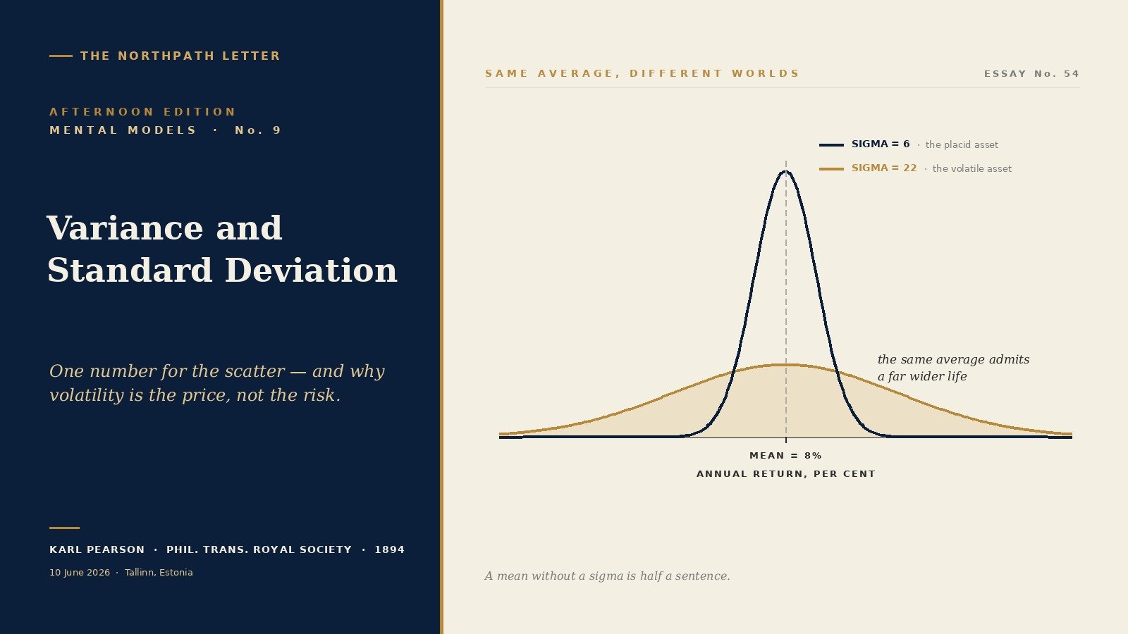
Why does the law work, and what makes it brittle? Consider a portfolio of n independent and identically distributed positions whose individual return X has finite expectation μ and finite variance σ². The arithmetic mean of the n positions is X̄_n = (X₁ + X₂ + … + X_n) / n. Two elementary facts about the distribution of X̄_n drive everything that follows. The expectation E[X̄_n] equals μ itself, irrespective of n: the expected value of the average is the true mean. The variance Var(X̄_n) equals σ² / n: the standard deviation of the average shrinks as 1/√n.

The shrinkage in 1/√n is the mathematical engine. Doubling the sample size reduces the standard error by a factor of √2, not 2. Quadrupling it halves the standard error. This is why convergence is real but slow: getting from a standard error of ten percent down to one percent requires a hundred-fold increase in sample size, not a ten-fold one. It is also why the most common quantitative claim in investing—”this strategy has worked over a five-year backtest”—is, in many cases, a single noisy observation rather than statistical evidence.

The mechanism rests on four assumptions, each of which is fragile in real markets. The first is the independence of draws: cross-correlated positions—every Indian small-cap, every European bank stock, every US high-multiple software name—do not provide n independent observations; they provide some smaller effective sample size n_eff. The second is identical distribution: if the underlying process changes over the sampling window—a regulatory regime change, a structural shift in interest rates, the entry of a new disruptive technology—what looks like one long sample is actually two short samples glued together. The third is finite expectation: for a few important investment-relevant distributions, notably power-law-tailed return distributions in the spirit of Mandelbrot (1963) and Taleb (2020), the theoretical mean exists but the sample mean converges very slowly; for distributions without finite variance, the central limit theorem fails altogether. The fourth is a long enough horizon: convergence is asymptotic, and at any finite n the sample average remains a random variable around the true mean.

Amos Tversky and Daniel Kahneman, in their 1971 paper “Belief in the Law of Small Numbers” (Psychological Bulletin, vol. 76, no. 2, pp. 105–110), documented that even trained statisticians systematically overestimate the reliability of small samples—they treat n = 20 as if it were the asymptotic case. The behavioural literature has replicated this finding many times since. For the investor, the takeaway is that the law of large numbers is silent at the sample sizes most investors care about; only the law of small numbers is operative.

3. The empirical record

The most striking empirical record of the law of large numbers in equity markets concerns the wide dispersion of individual stock returns and the consequently large sample sizes required before broad-market averages stabilise. Hendrik Bessembinder, in “Do Stocks Outperform Treasury Bills?” (Journal of Financial Economics, vol. 129, 2018, pp. 440–457), computed lifetime returns for the universe of CRSP US common stocks from 1926. Of roughly 26,000 individual stocks, just over half (51.6 per cent) delivered lifetime returns below those of one-month Treasury bills. The aggregate equity premium over Treasury bills since 1926 was driven by a small minority: the top 4 per cent of stocks accounted for the entirety of the net dollar wealth creation; the median stock destroyed wealth relative to T-bills. In the global update (Bessembinder, Chen, Choi & Wei, “Long-Term Shareholder Returns: Evidence from 64,000 Global Stocks,” SSRN working paper, 2023), 60.9 per cent of 64,000 international stocks underperformed cash over their lives.

Bessembinder’s numbers are the law of large numbers in operation. The market-cap-weighted aggregate is well-behaved because n is enormous—tens of thousands of names over a century, with very high effective sample size. The index-level mean reliably reflects the equity-premium expectation. But the same arithmetic implies that a portfolio of ten names is not a meaningful sample of the equity-return distribution. The standard error of the average return of ten randomly-drawn stocks is roughly thirty per cent of the true σ; for one hundred names it is roughly ten per cent. This is the source of Meir Statman’s “diversification ratio” empirical result (“How Many Stocks Make a Diversified Portfolio?”, Journal of Financial and Quantitative Analysis, vol. 22, no. 3, 1987, pp. 353–363): something on the order of thirty stocks captures most diversifiable variance, but residual idiosyncratic risk remains material.

The other empirical anchor is the S&P Indices Versus Active Funds (SPIVA) scorecard, published semi-annually since 2002. The SPIVA U.S. Mid-Year 2024 Scorecard reports that, over the fifteen-year window through June 2024, 89.9 per cent of large-cap actively-managed equity mutual funds underperformed the S&P 500. The single-year figure for the twelve months ended mid-2024 was around 57 per cent. The five-year figure was 77 per cent. As the horizon lengthens—as n grows—the dispersion in apparent skill compresses dramatically, and the share of funds that look skilful approaches the share that one would expect from pure noise net of the cost drag. Both data sources point to the same operating fact for the long-term equity investor: at short horizons, almost anything can happen in the sample mean; at long horizons, structural truths assert themselves. The discipline is not to confuse the two regimes.

4. Two historical episodes

4.1 The Nifty Fifty, 1968–1974

Through the late 1960s and into 1972, a roughly forty-stock set of US growth franchises—Polaroid, Eastman Kodak, Xerox, IBM, Avon, Coca-Cola, Johnson & Johnson, Procter & Gamble, McDonald’s, Disney—traded at price-earnings multiples between fifty and ninety, on the proposition that their durable growth justified essentially any starting multiple. The empirical evidence then cited was their immediate post-war record: roughly two decades of high and apparently stable earnings growth. The argument was framed as a long-run truth.

It was a short-run sample. The sample period chosen (1949–1969) was a unique structural episode: a US export franchise into a war-flattened world, the bedding-in of the post-war consumer economy, and a long disinflation. When the 1973–74 bear market began and the underlying stagflation revealed itself, the Nifty Fifty stocks fell forty to eighty per cent from peak; several—Polaroid, Avon, Eastman Kodak—never recovered their 1972 highs in real terms. Jeremy Siegel’s two retrospectives (“Valuing Growth Stocks: Revisiting the Nifty Fifty,” AAII Journal, October 1998, and “The Nifty Fifty Revisited,” Journal of Portfolio Management, vol. 21, 1995) showed that the basket as a whole did, eventually, justify its 1972 multiples over thirty years—but only as an aggregate, with extreme dispersion within the basket and decades of underwater holding for many individual names. The episode is the canonical example of treating a small, regime-specific sample as if it were the asymptotic case.

4.2 Long-Term Capital Management, 1994–1998

LTCM’s swap-spread and convergence trades were sized using volatility estimates from a roughly five-year sample of post-Maastricht European data, in which sovereign spreads had been gently grinding tighter. The bet was that the empirical volatility of that period was representative of the underlying process. Roger Lowenstein’s When Genius Failed (Random House, 2000) and Donald MacKenzie’s reconstruction in An Engine, Not a Camera (MIT Press, 2006, chapter 8) both document that LTCM’s leverage was calibrated to volatility numbers from a benign regime that excluded both the 1987 crash and the 1998 emerging-market crises that followed. When Russia defaulted on its rouble-denominated debt in August 1998, the realised volatility was an order of magnitude above the modelled volatility; the convergence trades widened rather than converged; and the fund—with capital of $4.7 billion at peak and notional positions over $1.25 trillion—required a $3.6 billion Fed-coordinated bailout to wind down without forcing a systemic event.

LTCM is not a story about the law of large numbers failing. It is a story about the assumption of stationarity failing. The sample size was, mathematically, adequate for narrow inference; what was inadequate was the assumption that the next draw came from the same distribution as the prior draws. Both episodes—the Nifty Fifty and LTCM—teach the same operating lesson: it is not n that matters, it is whether the n draws come from a distribution that resembles the distribution that will generate the next draw.

5. Application to long-term equity investing

Three operating disciplines follow directly from the law of large numbers for any investor with a multi-decade horizon.

Discipline 1: Concentrate, but ensure enough independent bets to let convergence work. A one-stock portfolio has, by construction, an effective sample size of one. The standard error of its annual return is the standard error of a single name—for individual stocks, that has historically been roughly thirty to fifty per cent per year (Bessembinder, 2018). A thirty-stock portfolio of well-diversified independent exposures has an effective n closer to thirty, and a sample-mean standard error roughly five to six times smaller. The trade-off between conviction (concentrate) and convergence (diversify) is genuine, but the relevant variable is effective n, not nominal n. Forty correlated bank stocks are still one bet. The right test for any new candidate is whether its primary economic exposure is materially different from the exposures already in the book.

Discipline 2: Demand long horizons before judging skill. The SPIVA data implies that even five-year returns provide weak evidence of skill, because the noise dominates the signal. The relevant unit of sample in investment skill is not the trade or the quarter but the cycle. Michael Mauboussin’s The Success Equation (Harvard Business Review Press, 2012) shows that for activities where luck plays a substantial role, the required sample size to detect a one-percentage-point edge with reasonable confidence is in the dozens of cycles, not the dozens of months. The honest implication is that an investor must judge their own process more by the discipline of the inputs (research depth, position sizing, behavioural restraint) than by the trailing returns of the outputs over any short window.

Discipline 3: Distinguish stationary from non-stationary processes before extrapolating. Most investment “rules”—sector beta, factor premia, sovereign spread relationships, currency mean-reversion—are stationarity assumptions wearing the costume of statistical inference. The questions to ask, before applying any historical relationship to capital, are: what regime produced this sample?, what would change the regime?, and would I notice the regime change in time? If the answers are unclear, the sample is short, and the prudent posture is humility about the inference. Warren Buffett’s 1996 owner’s manual injunction—that Berkshire avoids situations where it must “be precise about a number that we don’t really understand”—is, at its root, a statement about non-stationarity: when the data-generating process can shift in ways we cannot anticipate, no amount of historical data delivers asymptotic comfort.

These three disciplines do not produce a strategy. They produce a posture: the long-term equity investor is one who accepts that her edge is statistical, that statistical edges only manifest over many independent observations, and that the cost of forgetting this is the destruction of the very compounding she was trying to harvest.

6. How the long-term equity tradition has used it

Warren Buffett has invoked the law explicitly, if informally, throughout the Berkshire Hathaway chairman’s letters. In the 1991 chairman’s letter (Berkshire Hathaway Inc., 1991 Annual Report, dated 28 February 1992), Buffett described the insurance underwriting franchise as one whose results would, “with a long-enough horizon and a wide-enough underwriting book, revert to the underlying actuarial truth.” The thought is repeated, in different forms, in the 1996 owner’s manual and again in the 2014 letter marking Berkshire’s first fifty years: investment skill manifests across a sample of decades, not a sample of months. Berkshire’s own structure—permanent capital, no redemption pressure, a willingness to hold concentrated positions for thirty years—is engineered to let the law operate without interruption. The insurance float strategy in particular is a literal application of Bernoulli’s theorem: across a sufficiently large book of independent risks, the underwriting result converges to the underlying actuarial expectation, and the float earns a return in between.

Howard Marks has built much of his published thinking around the same statistical core. The Oaktree memo “Risk” (January 2006) frames investment risk as the distribution of possible outcomes around an expected value, and warns explicitly against treating a small realised sample as evidence about the distribution. In “How the Game Should Be Played” (Oaktree Capital, August 2017) and again in Mastering the Market Cycle (Houghton Mifflin Harcourt, 2018, chapter 1), Marks returns to the same point: a single year, a single trade, a single cycle is one draw from a wide distribution; the investor’s job is to think probabilistically about all the draws that could have happened, not just the one that did. Bernoulli’s theorem is the formal expression of why this discipline matters: the next draw is information, but it is not the truth.

Charles Ellis, in “The Loser’s Game” (Financial Analysts Journal, July–August 1975, pp. 19–26), made the same argument earlier and in stronger form. Ellis’s central observation was that the proliferation of professional investors and the falling cost of information had moved equity markets from a winner’s game (where skill systematically rewards itself in the short run) to a loser’s game (where the dominant variable is the cost of mistakes). The implication, framed in our terms: in a loser’s game, the long-run statistical result is determined by who can afford to wait for n to become large enough for the mean to assert itself, net of fees and frictions, and who has the temperament to resist acting on small-n signals. The rise of indexed and long-only patient capital in the four decades since is, in a sense, the institutional embodiment of Ellis’s reading of Bernoulli. The intellectual chain from Bernoulli to Ellis to Buffett to Marks is direct. It is not a chain about specific stock picks; it is a chain about what kind of evidence about investment skill it is rational to demand, and on what time scale.

7. Key takeaways

The law of large numbers is the formal justification for taking the long view, but it is silent on whether any particular sample is large enough. The honest investor decomposes “long-run” claims into a precise n and a precise assumption about stationarity. Standard error shrinks as 1/√n, not 1/n: doubling a sample halves the standard error by a factor of about 1.41, not 2, and most published track records are at sample sizes where most of the variation is still noise. Independent observations are the input—correlated positions are not; effective n in a portfolio is almost always materially below nominal n, and the first test of any new position is its marginal contribution to true independence. The Nifty Fifty and Long-Term Capital Management are the same mistake in different clothing: both treated a short, regime-specific sample as a description of the underlying process. The long-term equity tradition, from Bernoulli through Ellis to Buffett and Marks, has never been about predicting the next outcome; it has been about earning the right to wait for the law to operate.

— Manish Goel, FCA / NorthPath Advisory OÜ / Tallinn, Estonia

Important. All content on this site and in this email is journalism and education for a general audience. Nothing here constitutes investment advice or a recommendation in respect of any specific financial instrument, nor an offer or solicitation to buy or sell any security. Readers should consult an authorised financial adviser regulated in their own jurisdiction before making any investment decision.

Afternoon Edition — Mental Models · Essay No. 7 · 25 May 2026 · Tallinn

1. The model: a posthumous paper that quietly reorganised how we should think

Thomas Bayes was a Presbyterian minister and amateur mathematician who lived in Tunbridge Wells and died in 1761. He published almost nothing in his lifetime. Two years after his death, his friend Richard Price submitted his notes to the Royal Society. The paper appeared in 1763 under the unassuming title An Essay towards solving a Problem in the Doctrine of Chances, in volume 53 of the Philosophical Transactions, pages 370 to 418. It was largely ignored for the next century and a half.

What Bayes had derived, and what Pierre-Simon Laplace independently restated in cleaner form in 1774 and 1812, was a rule for updating a belief in light of new evidence. In modern notation the rule is one line. The probability of a hypothesis H given new data D equals the probability of H before seeing D, multiplied by the probability that D would have occurred if H were true, divided by the unconditional probability of D itself. Or, in the form an investor will use most often: posterior is proportional to prior times likelihood.

That single equation does several things at once. It tells you that your starting belief — your prior — matters and must be made explicit. It tells you that the diagnostic value of a piece of evidence is not its loudness but the ratio of how likely it is under the hypothesis you favour versus under the alternative. It tells you that updating is a multiplicative, not additive, operation, which means very strong evidence can swamp a prior and very weak evidence almost cannot. And it tells you that two reasonable people with different priors and the same evidence will, with enough rounds of updating, eventually converge on the same posterior. That last property is why long-term investors who think in Bayesian terms tend, over decades, to converge on similar judgments about the same business even when they started in very different places.

2. The mechanism: why it works, and where it breaks

The deeper claim of Bayes’ rule is that there is, up to a choice of prior, exactly one consistent way to revise probability assignments in the light of new information. Frank Ramsey proved a version of this in 1926, and Bruno de Finetti in 1937. Their argument is sometimes called the Dutch-book theorem: if your beliefs do not obey the laws of probability, a counterparty can in principle construct a sequence of bets you would accept that guarantees you a loss. To be coherent in the face of uncertainty is, definitionally, to update like a Bayesian.

The rule works because it forces three pieces of intellectual hygiene that human cognition naturally resists. First, you must state your prior before you see the new evidence. Most investors form an opinion about a company, then read its quarterly report, then claim the report confirmed an opinion they had pre-loaded. Bayes’ rule does not permit this. Second, you must specify what the data would look like under each rival hypothesis, not only under your favoured one. A flat results print can mean the business is dying, or that management is investing for the next cycle, or that a one-off accounting item has masked underlying strength. The Bayesian asks which of those worlds best explains what you see, weighted by how likely the data are in each. Third, you must update by the right magnitude. Strong likelihood ratios produce large updates; weak ones produce small updates; and a piece of evidence whose probability is roughly equal under all hypotheses produces no update at all, however dramatic it appears.

Where the rule breaks is at the prior. Bayes himself was uneasy on this point; Price was uneasier; Laplace papered over it with his principle of insufficient reason. In practice the prior is the place where craft enters. Two investors looking at the same Indian cement company can have very different priors about the trajectory of its return on capital because one has lived through the 1995 to 2003 cycle and one has not. Neither prior is wrong; they are conditioned on different lifetimes of data. What Bayes’ rule guarantees is only that, if both update honestly on the next ten years of evidence, their posteriors will move toward each other.

3. The empirical record

For most of two centuries Bayes’ rule sat in the corner of probability theory while the Neyman-Pearson frequentist school dominated statistics. The revival began with three strands of empirical evidence that frequentist methods were leaving systematic value on the table.

The first was in medical diagnosis. David Eddy, writing in the Journal of the American Medical Association in 1982, presented a now-famous problem to a group of physicians. A woman has a positive mammogram. The base-rate prevalence of breast cancer in her age group is roughly 1 per cent. The mammogram has a sensitivity of 80 per cent and a false-positive rate of about 10 per cent. What is the probability she has cancer? The correct Bayesian answer is around 7.5 per cent. The median answer from the physicians was 75 per cent. Gerd Gigerenzer and Ulrich Hoffrage replicated the result in 1995 across a larger sample of clinicians: most professionals confronted with a screening problem ignore the base rate almost entirely and read the positive test result as if it were the posterior, not the likelihood. The cost of this error, scaled across an entire health system, is measurable in tens of billions of dollars and thousands of unnecessary procedures every year.

The second strand is the IARPA Good Judgment Project, which ran from 2011 to 2015 under Philip Tetlock and Barbara Mellers. The project recruited several thousand volunteer forecasters to predict geopolitical and economic events: would Greece leave the Eurozone in the next year, would the Chinese exchange rate move outside a band, would a particular regime survive a coup attempt. Forecasters were scored using the Brier score, a proper rule that rewards both correctness and calibration. The top-performing 2 per cent, whom Tetlock labelled superforecasters, were not domain experts; they were Bayesian updaters. They wrote down explicit numerical priors, defined the events under which they would update, and moved their probability estimates in small increments — often by single percentage points — as new evidence arrived. Over four years they beat the average forecaster by 30 per cent and the average intelligence-community analyst by a margin that was politically embarrassing to publish.

The third strand is the academic re-examination of professional security analysts. Werner De Bondt and Richard Thaler, in Journal of Finance 1990, documented that sell-side analysts systematically over-react to recent earnings news — they update too far on weak evidence — and under-react to long-running shifts in fundamentals — they update too little on strong evidence. Subsequent work by Easterwood and Nutt in 1999 confirmed the pattern across multiple decades and markets. The error is not random; it is the exact opposite of what Bayes’ rule prescribes. Likelihood ratios that should produce a small movement produce a large one, and likelihood ratios that should be decisive produce almost no change.

4. Two historical episodes

The first is Bletchley Park, 1941 to 1945. Alan Turing arrived at the British codebreaking centre in September 1939 and within two years had built, with the help of the statistician I. J. Good, a Bayesian apparatus for breaking the daily key of the German naval Enigma. Their method, which Good later described in his 1979 paper Studies in the History of Probability and Statistics, was to maintain a running posterior on each candidate wheel setting and to update it message by message using the log-likelihood ratio between the candidate setting and a random one. The unit of evidence they used, the ban and the deciban, was simply log base ten of a likelihood ratio. Turing chose decibans because he had calibrated, through his own experience, that the human mind could meaningfully distinguish posterior odds at roughly that resolution. The system worked. From 1942 onward the British were reading German U-boat traffic in close to real time, and the Battle of the Atlantic turned. Sharon Bertsch McGrayne, in The Theory That Would Not Die (Yale 2011), estimates that the codebreaking shortened the war by two to four years and that the entire enterprise rested on Bayes’ rule applied with discipline.

The second is the search for the lost American hydrogen bomb off Palomares, Spain, in January 1966. A B-52 had collided with a refuelling tanker; four bombs fell, three on land, one into the Mediterranean. The US Navy needed to find it before the Soviets did. Dr John Craven, the Navy’s chief scientist on the deep-submergence program, assembled a panel of submarine commanders, weapons experts and oceanographers and asked each to construct a probability map for where the bomb had landed, conditional on what they knew about the aircraft’s trajectory, currents and impact dynamics. He then combined these priors using Bayes’ rule into a single posterior map and directed the search ships accordingly. As each grid square was searched and came up empty, he updated the map again, redistributing probability into the unsearched cells. The bomb was found, eighty days after impact, in a square that the consensus prior would have ranked low but that the Bayesian update had elevated to high posterior after several other squares came up clean. Craven repeated the method in 1968 to locate the lost submarine USS Scorpion, this time with even less data and even greater success. Both episodes are documented in Craven’s memoir The Silent War (Simon & Schuster, 2001) and in the McGrayne history cited above. They are the clearest demonstrations on record of how a properly applied Bayesian framework outperforms expert intuition on problems where the prior is uncertain and the evidence trickles in.

5. Application to long-term equity investing — three concrete disciplines

The first discipline is the written prior. Before reading a company’s annual report, the Bayesian investor writes down a numerical estimate of the probability that the business will earn a stated minimum return on capital over the next five years. The estimate is conditioned on what is already known: the industry’s long-run economics, the company’s reinvestment history, the calibre of its capital allocator, the regulatory regime. The number is not an idle guess; it is the prior against which every new disclosure will be weighed. If the prior is 60 per cent and the half-year results would have been roughly equally likely whether the underlying probability were 60 per cent or 50 per cent, the rational update is small. If the results contain a piece of information that is far more likely under the 60 per cent world than under the 50 per cent one — a structural margin expansion, say, that no competitor has matched — the update is large. Without the written prior there is nothing to update from, and the investor falls back on the recency-weighted heuristics that the De Bondt-Thaler studies show to be biased.

The second discipline is the likelihood-ratio table. For each significant operating metric the investor maintains a small table: what would the metric look like in a world where the business is genuinely improving; what would it look like in a world where management is engineering an appearance of improvement; what would it look like in a world where the underlying franchise is decaying. The same printed number — say, a 200 basis-point uptick in operating margin — has very different implications in each world. The investor’s job is not to debate whether the number is good or bad but to ask which of the three worlds best explains it, and to update accordingly. Michael Mauboussin, in More Than You Know (Columbia 2006), calls this thinking in expected value across scenarios rather than around a single point estimate; the structure is identical to Bayes’ rule applied scenario by scenario.

The third discipline is small steps. The Tetlock superforecasters did not change their estimates from 60 per cent to 20 per cent in a single move. They moved from 60 to 57 to 55 to 52, taking each piece of evidence at its true informational weight. The same applies in equity investing. A long-term holding worth holding at a 60 per cent posterior of meeting one’s hurdle is rarely worth selling outright on a single quarterly disappointment; it is worth re-marking the posterior downward by a few points and re-examining whether that change crosses any decision threshold. The opposite error — wholesale conviction reversal on a single data point — is exactly what Easterwood and Nutt found analysts doing, and exactly what the long-tail of equity returns demonstrated by Hendrik Bessembinder punishes most severely. The handful of stocks that produce the bulk of decade-long returns rarely advertise themselves with clean linear progress; they are noisy on the way to greatness, and a Bayesian who updates in small steps survives the noise.

6. How the long-term equity tradition has used it

Charles T. Munger, in his 1995 Harvard Law lecture The Psychology of Human Misjudgement, lists “the absence of an elementary probability calculation” as among the leading causes of investing failure. Five years later, in his 2000 commencement address at the USC Law School, he was more specific: “If you don’t get this elementary, but mildly unnatural, mathematics of elementary probability into your repertoire, then you go through a long life like a one-legged man in an ass-kicking contest. You’re giving a huge advantage to everybody else.” The probability calculation he had in mind was, in essence, Bayes’ rule: the requirement to combine a prior with a likelihood instead of reading new evidence as if it were itself the posterior.

Howard Marks has built much of his writing at Oaktree around the same idea, without always using the Bayesian vocabulary. In his memo of January 2014, Dare to Be Great II, he writes that the second-level investor is the one who asks not what the news means but how the news will change the consensus probability assignment to a range of outcomes — and how that change should differ from his own update. The arbitrage opportunity, in Marks’ framework, is the gap between the market’s likelihood ratio and one’s own better-calibrated one. The discipline that holds the framework together is the requirement to do the calculation explicitly. In The Most Important Thing (Columbia 2011) he devotes a chapter to the difference between knowing the range of outcomes, knowing their probabilities, and knowing how to update both as the world unfolds. That sequence — range, probability, update — is the Bayesian sequence stated in plain English.

Among practising portfolio managers the explicit case is Bill Miller, who ran the Legg Mason Value Trust from 1990 to 2012. Miller used a Bayesian decision framework — he had brought Mauboussin into the firm to build it — and the framework’s mathematics is what allowed him to hold positions in Amazon and Dell through drawdowns that conventional analysts treated as decisive evidence of impairment. Miller’s view was that the drawdowns were exactly the noisy evidence Bayes’ rule prescribes a small update for, not the catastrophic news that warranted abandonment. The framework eventually broke in 2008, not because Bayes’ rule failed, but because Miller’s prior on US financial-sector capital adequacy was anchored on a regime that had ended. The lesson there is the one McGrayne emphasises: Bayes’ rule is only as good as the honesty with which the prior is constructed, and a prior that does not update its own structural assumptions when the structure itself changes is no defence.

7. Key takeaways

Bayes’ rule is the algebra of changing one’s mind. Five operational consequences follow for the long-term equity investor.

One. Write the prior down before the data arrive. An unwritten prior is, by the time the data are in, indistinguishable from a rationalisation.

Two. For every important metric, ask what the data would look like under each rival hypothesis, not only under the favoured one. The diagnostic value of evidence is the ratio of those probabilities, not the loudness of the number.

Three. Update in small steps. A coherent Bayesian almost never moves the posterior by more than ten percentage points on a single quarter’s print. The investors who do so are advertising that they had no prior to begin with.

Four. Convergence is a feature, not a bug. Two analysts with different priors who both update honestly will, given enough rounds of disclosure, end up close to each other. If your view is moving away from informed others’ views over time, the prior is probably anchored on a fact pattern that no longer holds.

Five. The prior is where the craft lives. The arithmetic of updating is mechanical; the choice of prior is judgment. Most of what experienced investors learn over decades is encoded in better priors, not in better updates. The error that ends most careers is a stale prior that refuses to be re-examined when the structural facts change underneath it.

Bayes’ rule will not tell anyone which company to own. It will, applied honestly, prevent the investor from being so easily moved by the latest piece of evidence that they are still being moved by it when the next, contradictory, piece arrives. In a profession whose hardest task is to do less in response to noise, that is a service whose value is hard to overstate.

— Manish Goel, FCA / NorthPath Advisory OÜ / Tallinn, Estonia

Important. All content on this site and in this email is journalism and education for a general audience. Nothing here constitutes investment advice or a recommendation in respect of any specific financial instrument, nor an offer or solicitation to buy or sell any security. Readers should consult an authorised financial adviser regulated in their own jurisdiction before making any investment decision.