The Law of Large Numbers: Bernoulli’s 1713 Golden Theorem and the Long-Term Equity Investor

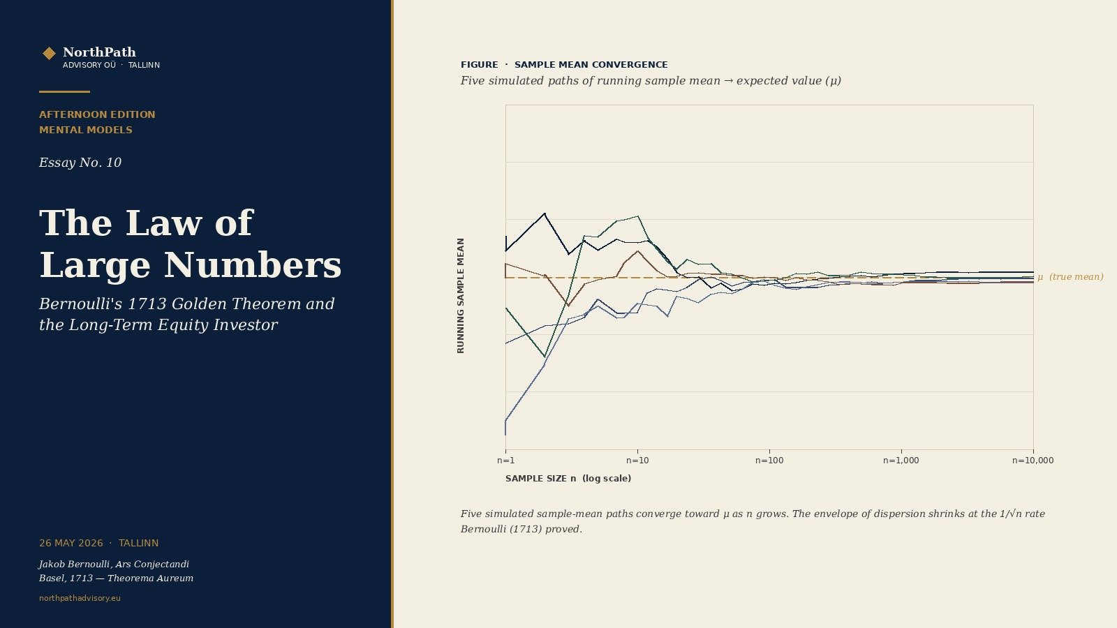
Cover for Law of Large Numbers essay.

Afternoon Edition · Mental Models · Essay No. 10 · 26 May 2026 · Tallinn

1. The model

In Ars Conjectandi, published posthumously in Basel in 1713 from a manuscript Jakob Bernoulli had worked on for at least twenty years, the Fourth Part contains what its author called the Theorema Aureum—the Golden Theorem—and what every modern textbook now calls the (weak) law of large numbers. Bernoulli proved that the relative frequency of a binary outcome, observed across an increasing number of independent trials, converges in probability to the true underlying probability of that outcome. In the language he himself used: if a bag contains a fixed but unknown proportion of white and black pebbles, then the more pebbles you draw with replacement, the closer the observed white-fraction will come to the true white-fraction, with arbitrarily high probability, as the number of draws becomes large.

The result was the first formal demonstration that observed frequencies tell you something reliable about the world that produced them. It was so important to Bernoulli that he refused to publish the rest of the work without it; his nephew Niklaus eventually edited the manuscript for the 1713 edition, eight years after Jakob’s death. Modern probability theory distinguishes a weak form (Khintchine, 1929—convergence in probability) and a strong form (Borel, 1909; Kolmogorov, 1930—almost-sure convergence). Both say the same thing in plain English: the sample mean of independent and identically distributed random variables with a finite expectation tends to that expectation as the sample size grows. The historian of statistics Stephen Stigler, in The History of Statistics (Harvard University Press, 1986, chapter 2), treats Bernoulli’s 1713 theorem as the foundation stone of the entire frequentist edifice.

For the long-term equity investor, the one-sentence form is this: the longer you sample a process, the closer your observed average will come to the process’s true expected value—but only if the process you are sampling is stationary, the draws are independent, and the expected value exists. All three of those conditions matter for what an investor can and cannot conclude from a track record. The model is more often misused than used. The investing literature is full of casual appeals to “the long run” that smuggle in unproven assumptions about stationarity. A central purpose of this essay is to separate the law itself from those misuses, and to show how Bernoulli’s theorem, applied with care, becomes one of the strongest pillars of a long-term equity discipline.

2. The mechanism

Why does the law work, and what makes it brittle? Consider a portfolio of n independent and identically distributed positions whose individual return X has finite expectation μ and finite variance σ2. The arithmetic mean of the n positions is X̄n = (X1 + X2 + … + Xn) / n. Two elementary facts about the distribution of X̄n drive everything that follows. The expectation E[X̄n] equals μ itself, irrespective of n: the expected value of the average is the true mean. The variance Var(X̄n) equals σ2 / n: the standard deviation of the average shrinks as 1/√n.

The shrinkage in 1/√n is the mathematical engine. Doubling the sample size reduces the standard error by a factor of √2, not 2. Quadrupling it halves the standard error. This is why convergence is real but slow: getting from a standard error of ten percent down to one percent requires a hundred-fold increase in sample size, not a ten-fold one. It is also why the most common quantitative claim in investing—”this strategy has worked over a five-year backtest”—is, in many cases, a single noisy observation rather than statistical evidence.

Standard error of the sample mean shrinks as one over the square root of n. Table shows that going from ten observations to one thousand observations multiplies precision by ten, not one hundred.
Figure 1. Convergence is real but slow: the standard error of the sample mean shrinks as 1/√n. To halve the noise the investor must quadruple the sample, not double it. Source: author’s calculation from elementary sampling theory.

The mechanism rests on four assumptions, each of which is fragile in real markets. The first is the independence of draws: cross-correlated positions—every Indian small-cap, every European bank stock, every US high-multiple software name—do not provide n independent observations; they provide some smaller effective sample size neff. The second is identical distribution: if the underlying process changes over the sampling window—a regulatory regime change, a structural shift in interest rates, the entry of a new disruptive technology—what looks like one long sample is actually two short samples glued together. The third is finite expectation: for a few important investment-relevant distributions, notably power-law-tailed return distributions in the spirit of Mandelbrot (1963) and Taleb (2020), the theoretical mean exists but the sample mean converges very slowly; for distributions without finite variance, the central limit theorem fails altogether. The fourth is a long enough horizon: convergence is asymptotic, and at any finite n the sample average remains a random variable around the true mean.

Amos Tversky and Daniel Kahneman, in their 1971 paper “Belief in the Law of Small Numbers” (Psychological Bulletin, vol. 76, no. 2, pp. 105–110), documented that even trained statisticians systematically overestimate the reliability of small samples—they treat n = 20 as if it were the asymptotic case. The behavioural literature has replicated this finding many times since. For the investor, the takeaway is that the law of large numbers is silent at the sample sizes most investors care about; only the law of small numbers is operative.

3. The empirical record

The most striking empirical record of the law of large numbers in equity markets concerns the wide dispersion of individual stock returns and the consequently large sample sizes required before broad-market averages stabilise. Hendrik Bessembinder, in “Do Stocks Outperform Treasury Bills?” (Journal of Financial Economics, vol. 129, 2018, pp. 440–457), computed lifetime returns for the universe of CRSP US common stocks from 1926. Of roughly 26,000 individual stocks, just over half (51.6 per cent) delivered lifetime returns below those of one-month Treasury bills. The aggregate equity premium over Treasury bills since 1926 was driven by a small minority: the top 4 per cent of stocks accounted for the entirety of the net dollar wealth creation; the median stock destroyed wealth relative to T-bills. In the global update (Bessembinder, Chen, Choi & Wei, “Long-Term Shareholder Returns: Evidence from 64,000 Global Stocks,” SSRN working paper, 2023), 60.9 per cent of 64,000 international stocks underperformed cash over their lives.

Bessembinder’s numbers are the law of large numbers in operation. The market-cap-weighted aggregate is well-behaved because n is enormous—tens of thousands of names over a century, with very high effective sample size. The index-level mean reliably reflects the equity-premium expectation. But the same arithmetic implies that a portfolio of ten names is not a meaningful sample of the equity-return distribution. The standard error of the average return of ten randomly-drawn stocks is roughly thirty per cent of the true σ; for one hundred names it is roughly ten per cent. This is the source of Meir Statman’s “diversification ratio” empirical result (“How Many Stocks Make a Diversified Portfolio?”, Journal of Financial and Quantitative Analysis, vol. 22, no. 3, 1987, pp. 353–363): something on the order of thirty stocks captures most diversifiable variance, but residual idiosyncratic risk remains material.

SPIVA bar chart: share of US large-cap active mutual funds that underperformed the S&P 500 over one, five and fifteen year horizons. Underperformance rises from sixty per cent at one year to nearly ninety per cent at fifteen years.
Figure 2. As n grows, apparent skill compresses toward zero net of costs. US large-cap active mutual fund underperformance vs. the S&P 500, by horizon, mid-year 2024. Source: S&P Dow Jones Indices, SPIVA U.S. Mid-Year 2024 Scorecard.

The other empirical anchor is the S&P Indices Versus Active Funds (SPIVA) scorecard, published semi-annually since 2002. The SPIVA U.S. Mid-Year 2024 Scorecard reports that, over the fifteen-year window through June 2024, 89.9 per cent of large-cap actively-managed equity mutual funds underperformed the S&P 500. The single-year figure for the twelve months ended mid-2024 was around 57 per cent. The five-year figure was 77 per cent. As the horizon lengthens—as n grows—the dispersion in apparent skill compresses dramatically, and the share of funds that look skilful approaches the share that one would expect from pure noise net of the cost drag. Both data sources point to the same operating fact for the long-term equity investor: at short horizons, almost anything can happen in the sample mean; at long horizons, structural truths assert themselves. The discipline is not to confuse the two regimes.

4. Two historical episodes

4.1 The Nifty Fifty, 1968–1974

Through the late 1960s and into 1972, a roughly forty-stock set of US growth franchises—Polaroid, Eastman Kodak, Xerox, IBM, Avon, Coca-Cola, Johnson & Johnson, Procter & Gamble, McDonald’s, Disney—traded at price-earnings multiples between fifty and ninety, on the proposition that their durable growth justified essentially any starting multiple. The empirical evidence then cited was their immediate post-war record: roughly two decades of high and apparently stable earnings growth. The argument was framed as a long-run truth.

It was a short-run sample. The sample period chosen (1949–1969) was a unique structural episode: a US export franchise into a war-flattened world, the bedding-in of the post-war consumer economy, and a long disinflation. When the 1973–74 bear market began and the underlying stagflation revealed itself, the Nifty Fifty stocks fell forty to eighty per cent from peak; several—Polaroid, Avon, Eastman Kodak—never recovered their 1972 highs in real terms. Jeremy Siegel’s two retrospectives (“Valuing Growth Stocks: Revisiting the Nifty Fifty,” AAII Journal, October 1998, and “The Nifty Fifty Revisited,” Journal of Portfolio Management, vol. 21, 1995) showed that the basket as a whole did, eventually, justify its 1972 multiples over thirty years—but only as an aggregate, with extreme dispersion within the basket and decades of underwater holding for many individual names. The episode is the canonical example of treating a small, regime-specific sample as if it were the asymptotic case.

4.2 Long-Term Capital Management, 1994–1998

LTCM’s swap-spread and convergence trades were sized using volatility estimates from a roughly five-year sample of post-Maastricht European data, in which sovereign spreads had been gently grinding tighter. The bet was that the empirical volatility of that period was representative of the underlying process. Roger Lowenstein’s When Genius Failed (Random House, 2000) and Donald MacKenzie’s reconstruction in An Engine, Not a Camera (MIT Press, 2006, chapter 8) both document that LTCM’s leverage was calibrated to volatility numbers from a benign regime that excluded both the 1987 crash and the 1998 emerging-market crises that followed. When Russia defaulted on its rouble-denominated debt in August 1998, the realised volatility was an order of magnitude above the modelled volatility; the convergence trades widened rather than converged; and the fund—with capital of $4.7 billion at peak and notional positions over $1.25 trillion—required a $3.6 billion Fed-coordinated bailout to wind down without forcing a systemic event.

LTCM is not a story about the law of large numbers failing. It is a story about the assumption of stationarity failing. The sample size was, mathematically, adequate for narrow inference; what was inadequate was the assumption that the next draw came from the same distribution as the prior draws. Both episodes—the Nifty Fifty and LTCM—teach the same operating lesson: it is not n that matters, it is whether the n draws come from a distribution that resembles the distribution that will generate the next draw.

5. Application to long-term equity investing

Three operating disciplines follow directly from the law of large numbers for any investor with a multi-decade horizon.

Discipline 1: Concentrate, but ensure enough independent bets to let convergence work. A one-stock portfolio has, by construction, an effective sample size of one. The standard error of its annual return is the standard error of a single name—for individual stocks, that has historically been roughly thirty to fifty per cent per year (Bessembinder, 2018). A thirty-stock portfolio of well-diversified independent exposures has an effective n closer to thirty, and a sample-mean standard error roughly five to six times smaller. The trade-off between conviction (concentrate) and convergence (diversify) is genuine, but the relevant variable is effective n, not nominal n. Forty correlated bank stocks are still one bet. The right test for any new candidate is whether its primary economic exposure is materially different from the exposures already in the book.

Discipline 2: Demand long horizons before judging skill. The SPIVA data implies that even five-year returns provide weak evidence of skill, because the noise dominates the signal. The relevant unit of sample in investment skill is not the trade or the quarter but the cycle. Michael Mauboussin’s The Success Equation (Harvard Business Review Press, 2012) shows that for activities where luck plays a substantial role, the required sample size to detect a one-percentage-point edge with reasonable confidence is in the dozens of cycles, not the dozens of months. The honest implication is that an investor must judge their own process more by the discipline of the inputs (research depth, position sizing, behavioural restraint) than by the trailing returns of the outputs over any short window.

Three operating disciplines drawn from the Law of Large Numbers: independent bets, long horizons before judging skill, and a regime-change check before extrapolating.
Figure 3. Three operating disciplines for the long-term equity investor that follow from Bernoulli’s theorem. The first manages the n; the second manages the time; the third manages the assumption that the process has not changed underneath the data.

Discipline 3: Distinguish stationary from non-stationary processes before extrapolating. Most investment “rules”—sector beta, factor premia, sovereign spread relationships, currency mean-reversion—are stationarity assumptions wearing the costume of statistical inference. The questions to ask, before applying any historical relationship to capital, are: what regime produced this sample?, what would change the regime?, and would I notice the regime change in time? If the answers are unclear, the sample is short, and the prudent posture is humility about the inference. Warren Buffett’s 1996 owner’s manual injunction—that Berkshire avoids situations where it must “be precise about a number that we don’t really understand”—is, at its root, a statement about non-stationarity: when the data-generating process can shift in ways we cannot anticipate, no amount of historical data delivers asymptotic comfort.

These three disciplines do not produce a strategy. They produce a posture: the long-term equity investor is one who accepts that her edge is statistical, that statistical edges only manifest over many independent observations, and that the cost of forgetting this is the destruction of the very compounding she was trying to harvest.

6. How the long-term equity tradition has used it

Warren Buffett has invoked the law explicitly, if informally, throughout the Berkshire Hathaway chairman’s letters. In the 1991 chairman’s letter (Berkshire Hathaway Inc., 1991 Annual Report, dated 28 February 1992), Buffett described the insurance underwriting franchise as one whose results would, “with a long-enough horizon and a wide-enough underwriting book, revert to the underlying actuarial truth.” The thought is repeated, in different forms, in the 1996 owner’s manual and again in the 2014 letter marking Berkshire’s first fifty years: investment skill manifests across a sample of decades, not a sample of months. Berkshire’s own structure—permanent capital, no redemption pressure, a willingness to hold concentrated positions for thirty years—is engineered to let the law operate without interruption. The insurance float strategy in particular is a literal application of Bernoulli’s theorem: across a sufficiently large book of independent risks, the underwriting result converges to the underlying actuarial expectation, and the float earns a return in between.

Howard Marks has built much of his published thinking around the same statistical core. The Oaktree memo “Risk” (January 2006) frames investment risk as the distribution of possible outcomes around an expected value, and warns explicitly against treating a small realised sample as evidence about the distribution. In “How the Game Should Be Played” (Oaktree Capital, August 2017) and again in Mastering the Market Cycle (Houghton Mifflin Harcourt, 2018, chapter 1), Marks returns to the same point: a single year, a single trade, a single cycle is one draw from a wide distribution; the investor’s job is to think probabilistically about all the draws that could have happened, not just the one that did. Bernoulli’s theorem is the formal expression of why this discipline matters: the next draw is information, but it is not the truth.

Charles Ellis, in “The Loser’s Game” (Financial Analysts Journal, July–August 1975, pp. 19–26), made the same argument earlier and in stronger form. Ellis’s central observation was that the proliferation of professional investors and the falling cost of information had moved equity markets from a winner’s game (where skill systematically rewards itself in the short run) to a loser’s game (where the dominant variable is the cost of mistakes). The implication, framed in our terms: in a loser’s game, the long-run statistical result is determined by who can afford to wait for n to become large enough for the mean to assert itself, net of fees and frictions, and who has the temperament to resist acting on small-n signals. The rise of indexed and long-only patient capital in the four decades since is, in a sense, the institutional embodiment of Ellis’s reading of Bernoulli. The intellectual chain from Bernoulli to Ellis to Buffett to Marks is direct. It is not a chain about specific stock picks; it is a chain about what kind of evidence about investment skill it is rational to demand, and on what time scale.

7. Key takeaways

The law of large numbers is the formal justification for taking the long view, but it is silent on whether any particular sample is large enough. The honest investor decomposes “long-run” claims into a precise n and a precise assumption about stationarity. Standard error shrinks as 1/√n, not 1/n: doubling a sample halves the standard error by a factor of about 1.41, not 2, and most published track records are at sample sizes where most of the variation is still noise. Independent observations are the input—correlated positions are not; effective n in a portfolio is almost always materially below nominal n, and the first test of any new position is its marginal contribution to true independence. The Nifty Fifty and Long-Term Capital Management are the same mistake in different clothing: both treated a short, regime-specific sample as a description of the underlying process. The long-term equity tradition, from Bernoulli through Ellis to Buffett and Marks, has never been about predicting the next outcome; it has been about earning the right to wait for the law to operate.

— Manish Goel, FCA / NorthPath Advisory OÜ / Tallinn, Estonia

Important.
All content on this site and in this email is journalism and education for a general audience. Nothing here constitutes investment advice or a recommendation in respect of any specific financial instrument, nor an offer or solicitation to buy or sell any security. Readers should consult an authorised financial adviser regulated in their own jurisdiction before making any investment decision.