Category: Value Investing

The NorthPath Letter · Value Investing · Morning Edition · 28 May 2026

In the 1973 fourth edition of The Intelligent Investor, Benjamin Graham did something most authors of investment classics never do. He wrote a chapter that any reader could mechanically apply on a Saturday afternoon, at any kitchen table, in any country, against any equity market, without consulting a broker, an analyst, or a chart. He called it “Stock Selection for the Defensive Investor” (Chapter 14). It contained seven numerical tests — size, balance-sheet strength, earnings stability, dividend record, earnings growth, price-to-earnings ratio, and price-to-book ratio. A stock that survived all seven was, in Graham’s words, a candidate for a portfolio that the investor could hold “without losing sleep and without paying close attention.”

The seven tests are not a stock-picking system in the modern sense. They are a filter on the population of listed equities, designed to leave behind only those for which the probability of a permanent loss of capital over a multi-year holding period is structurally low. The screen does not promise outperformance. It promises that you have begun the process of analysis from a universe in which most of the worst outcomes have already been excluded. That is a strikingly modest claim. It is also, in our experience after twenty-two years of practising the discipline, the only claim about a stock screen that does not eventually break.

1. The principle

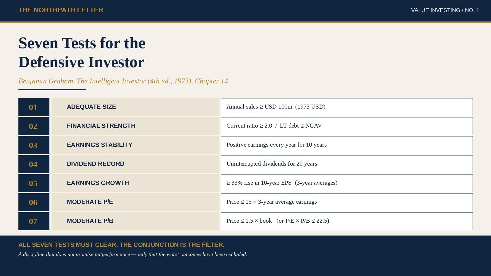
Graham defined the “defensive investor” as someone “whose chief emphasis will be on the avoidance of serious mistakes or losses; second goal, on freedom from effort, annoyance, and the need for making frequent decisions.” The seven tests were the operational expression of that definition. Each test sets a numerical minimum (or maximum) that a candidate stock must clear. The thresholds, in Graham’s 1973 wording, were:

Test 1 — Adequate size. Annual sales of at least USD 100 million (or, for a public utility, total assets of at least USD 50 million). Graham noted explicitly that this threshold was conservative even in 1973 and that “the result is to exclude small companies which may have unusual vicissitudes.” In 2026 currency, USD 100 million of 1973 sales is approximately USD 700 million to USD 1 billion of inflation-adjusted sales. We will return to this translation problem.

Test 2 — Sufficiently strong financial condition. Two sub-tests, both of which must clear: current ratio of at least 2.0, and long-term debt no greater than the net current asset value (current assets minus all liabilities). Together these put a hard floor under the company’s ability to survive a working-capital squeeze or a refinancing crisis without resort to equity dilution.

Test 3 — Earnings stability. Some earnings for the common stock in each of the past ten years. Note the precise wording: not earnings growth, not consistent returns on capital, simply positive reported earnings every year for a decade. The criterion excludes cyclicals at the peak of their cycle and start-ups that have not yet earned across a full business cycle.

Test 4 — Dividend record. Uninterrupted payments for at least the past twenty years. Graham’s deepest test, and the one that, in our work today, narrows the qualifying universe more aggressively than any other. A twenty-year unbroken dividend record is corroborating evidence that reported earnings have, over two decades, been backed by free cash flow large enough to support a payout through wars, recessions, and changes of management.

Test 5 — Earnings growth. A minimum increase of at least one-third in per-share earnings over the past ten years, using three-year averages at the beginning and end. The three-year averaging is the part most modern screens drop, and it is the part that does the real protective work: it removes the influence of cyclical peaks at either endpoint.

Test 6 — Moderate price-to-earnings ratio. Current price not more than fifteen times average earnings of the past three years.

Test 7 — Moderate price-to-asset ratio. Current price not more than one and one-half times the most recently reported book value. Graham added a softening clause: a lower P/E may justify a higher P/B, and a lower P/B may justify a higher P/E, provided the product of the two multiples does not exceed 22.5. That product test is the origin of what later authors christened “the Graham Number.”

Seven tests. Each test is a number. Each number is verifiable from the audited annual report. The screen requires no access to management, no proprietary database, no view on macroeconomic conditions, and no judgement about industry attractiveness. Graham’s deliberate intention was to construct a filter that a non-expert could apply, that an expert could not improve upon by adding intuition, and that would, in his words, “not leave the investor much exposed to the dangers of the market.”

2. The mechanism — why seven independent filters work

The intellectual content of the seven tests lies not in any single criterion but in their conjunction. Each criterion in isolation is unremarkable. A P/E below fifteen, a P/B below one and a half, a current ratio of two, a dividend record — in any modern stock screener these are standard fields. What makes the Graham screen different is that it requires all seven to clear simultaneously, and the criteria are constructed so that they fail on different kinds of company.

Consider the failure modes. A young company with no operating history fails tests 3 (ten-year earnings) and 4 (twenty-year dividend). A cyclical at the top of its cycle fails test 5 (three-year-averaged growth) and probably test 7 (P/B will be elevated). A leveraged roll-up fails test 2 (long-term debt versus net current assets). A declining business with melting earnings fails test 5 (growth measured between three-year averages). A glamour stock at the top of a bull market fails tests 6 and 7 (P/E and P/B). A capital-light business that has spent the last decade returning cash via buy-backs rather than dividends fails test 4. A small-cap with limited analyst coverage fails test 1.

The seven tests are therefore not redundant. They cover seven distinct sources of permanent capital impairment. The probability that a single stock passes all seven by accident is much lower than the product of the seven individual pass probabilities, because the conditions that produce high scores on one test (cheap multiples, for instance) tend to correlate negatively with the conditions that produce high scores on another (long dividend records, strong balance sheets). The conjunction is, statistically, a powerful filter.

This is why subset versions of the screen — “Graham’s low-P/E screen,” “the Graham Number screen,” “deep-value screens” that drop tests 3 through 5 — tend to perform worse than the full seven over multi-decade windows. Removing any one of the seven dilutes the filter’s ability to exclude a specific failure mode.

3. The empirical record

The most thorough academic test of Graham’s seven criteria remains Henry Oppenheimer’s “A Test of Ben Graham’s Stock Selection Criteria,” published in the Financial Analysts Journal, September–October 1984. Oppenheimer applied subsets of Graham’s criteria to all stocks traded on the New York and American Stock Exchanges between 1974 and 1981 and computed the realised total return of equally weighted portfolios formed from each subset. The full seven-criteria portfolio produced an arithmetic mean return of approximately 26 percent per annum over the eight-year period, against approximately 14 percent for the equally weighted CRSP universe. The premium was not driven by a single year; the seven-criteria portfolio outperformed the broad market in seven of the eight years.

Subsequent academic work has corroborated the result while disentangling the source of the excess return. Cliff Asness, Andrea Frazzini, and Lasse Pedersen of AQR Capital Management, writing in their 2015 paper “Quality Minus Junk,” reconstruct a measurable “quality” factor from criteria closely related to Graham’s tests 2 through 5 — profitability, growth, safety, and payout — and find that this quality factor has produced positive returns across twenty-four developed-market equity indices since the early 1980s. The Asness factor is not identical to Graham’s screen, but the overlap is substantial. The economic content of the seven tests has not decayed.

Jason Zweig’s 2003 commentary in the revised edition of The Intelligent Investor ran the seven-criteria filter against the US equity universe of the early 2000s and produced a sobering finding: the criteria, applied strictly, narrowed the universe to fewer than fifty stocks at most points in the 1995–2002 period. That is, in our view, a feature, not a defect. The screen is supposed to produce a small qualifying universe. A screen that produces five hundred candidates is no longer a filter; it is the market.

It is worth being precise about what the empirical record claims. The seven criteria do not promise that any individual stock passing them will outperform. They claim that, applied as a portfolio formation rule across many years and many regions, the resulting basket has historically produced returns above the market with downside volatility no higher than the market. That is the only claim a defensive screen is meant to make. It has, on the evidence, made it consistently.

4. Two historical episodes

The seven tests are designed to be applied in any market, in any year, but their character is most clearly visible in environments where the qualifying universe either expands or contracts dramatically.

The United States, 1974. The bear market of 1973–74 cut the S&P 500 by roughly 46 percent peak-to-trough and was the deepest equity drawdown since the 1930s. Graham’s fourth-edition revision was published in the middle of that bear market. He wrote in the new chapter that “the recent market decline has produced, for the first time in many years, a substantial number of stocks that meet our criteria.” Oppenheimer’s 1984 study, which began its sample period in 1974, captured exactly this moment. A defensive investor who applied the seven tests in 1974 and held the resulting portfolio for the next decade compounded at roughly twice the rate of the market while taking less drawdown risk. The screen was not predicting the 1975 recovery. It was simply identifying the population of stocks for which the probability of survival was high and the price paid was modest. Survival and modest price did the work.

Japan, 1990–2003. After the Nikkei 225 peaked at 38,915 in December 1989 and proceeded to fall to under 8,000 by 2003, the Japanese equity universe became, for over a decade, the global home of the Graham defensive screen. The combination of a long bear market, a culture of strong balance sheets and high cash balances, twenty-year-plus dividend histories at large industrial groups, and price-to-book ratios systematically below 1.0 across hundreds of companies produced more seven-criteria qualifiers than any market in financial history. The screen was widely written about in international value newsletters during these years (Marc Faber’s Gloom, Boom & Doom Report, Tweedy Browne’s investor letters, Fidelity’s overseas analyst notes), and the period offered an unusually clean test of the discipline: an investor who applied the seven tests to Japanese equities in 2003 and reinvested dividends would have substantially out-compounded the Topix index over the subsequent fifteen years. The discipline travelled. It did not need American conditions to work.

The two episodes are useful precisely because they look so different at the surface. The 1974 case is a normal cyclical bear market in the world’s deepest capital market. The Japanese case is a sui generis fifteen-year deflationary unwinding. The screen produced qualifying baskets in both, and the qualifying baskets produced acceptable long-term returns in both. A discipline that works only in one market structure is brittle. The seven tests, on this evidence, are not brittle.

5. The application framework — three practitioner disciplines

First, apply the criteria additively, not selectively. The seven tests are a logical conjunction. They are not a buffet from which the investor may pick the four that look most attractive in the current regime. We see this error frequently: investors retain tests 6 and 7 (cheap multiples) because the result feels concrete, drop tests 3 and 4 (earnings stability, dividend record) because they feel old-fashioned, and end up holding cyclicals near the top of their cycles. The screen’s protective character disappears entirely when the conjunction is broken. The discipline is binary: either all seven, or none of them as Graham intended.

Second, translate the formula to the holding period. Test 5 measures ten-year earnings growth using three-year averages at the beginning and end. That is a thirteen-year measurement window. The screen was not designed for monthly turnover. An investor who applies the seven tests with the intention of trading the resulting basket over twelve months is applying a screen calibrated for a different problem. Practitioners we respect — Walter Schloss, Tweedy Browne, the partners at Marathon Asset Management — have historically held the median position for three to seven years. The screen has a natural holding period embedded in its arithmetic, and an investor whose horizon is shorter than that horizon should expect the screen to underperform for them.

Third, adjust the size threshold to today’s units, not to today’s stories. The USD 100 million sales threshold of 1973 is roughly USD 700 million to USD 1 billion in inflation-adjusted 2026 terms. It is not a small-cap threshold. Graham himself wrote that the size criterion was the “weakest” of the seven and could be relaxed safely by an investor capable of doing additional balance-sheet work on smaller companies. Tests 2 through 5, by contrast, must not be relaxed. If a candidate company has only seven years of positive earnings rather than ten, the candidate does not pass test 3, and the response is not to lower the threshold — it is to wait three years, or to look at a different company. The numerical thresholds are the discipline; relaxing them is the equivalent of moving a goalpost.

6. How practitioners actually applied it

The seven tests have been used by serious long-term equity investors for more than five decades. Two case studies illustrate how the discipline survives in real portfolios.

Walter Schloss (Walter J. Schloss Associates, 1955–2002). Schloss was a junior analyst at the Graham–Newman Corporation in the late 1940s and went on to run an investment partnership for forty-seven years applying a Graham-style screen. His audited returns, published in Buffett’s 1984 Columbia Business School address “The Superinvestors of Graham-and-Doddsville,” show 15.7 percent annual gross returns over the 1955–1983 period against 11.2 percent for the S&P 500. Schloss did not apply all seven tests mechanically; he placed primary weight on tests 2 (financial strength), 3 (earnings stability), and 7 (price-to-book), with the price-to-book test acting as the binding constraint. He held an unusually large number of positions — often a hundred or more — precisely because his criteria produced a steady stream of qualifying candidates and he refused to concentrate. Schloss ’s case is instructive because it shows that the seven tests can be customised to a practitioner’s temperament without losing their protective character, provided the conjunction of strength, stability, and price remains intact.

Tweedy, Browne Partners (founded 1920, value-investing house since 1959). Tweedy Browne’s 1992 (updated 2009) white paper “What Has Worked in Investing” is the most thorough academic-style retrospective of Graham-style criteria from a practising firm. The paper compiles forty-four separate empirical studies of Graham-derived screens applied across the United States, the United Kingdom, Continental Europe, and Japan from the 1930s through the 2000s. The conclusion is, in our reading, the single most useful sentence written about the seven tests: “Investments characterised by some combination of low price relative to current asset value, low price-to-earnings ratios, low price-to-book ratios, significant insider buying, and consistent dividend records have produced returns substantially above the broad equity market over long measurement periods in every developed market studied.” The firm itself has applied a near-Graham screen to its Global Value Fund since 1993 with audited returns broadly in line with global equity benchmarks while taking materially lower drawdown.

The two firms’ experience converges on the same conclusion. The seven tests are robust to customisation, robust to market structure, and robust to changes in the underlying economy. They are not robust to dilution — that is, to the practice of dropping inconvenient tests — and they are not robust to a holding period shorter than the measurement window they were designed for.

7. Key takeaways

The defensive investor’s seven tests are a single discipline, not seven separate ones. The conjunction is the filter; dropping any test breaks it.

The screen was designed in 1973 for a holding period of five to ten years. Applying it on a shorter horizon transfers the screen’s benefit to someone else.

The qualifying universe will be small — tens of stocks in a normal market, hundreds in a bear market, near-zero at the top of a bull market. A wide qualifying universe is not a feature; it is a signal that the discipline is being relaxed.

The thresholds (current ratio of two, twenty-year dividend record, ten-year earnings, P/E of fifteen, P/B of one and a half) are not arbitrary. Each test addresses a specific failure mode. Adjustments to the size threshold for inflation are defensible. Adjustments to the others are not.

The seven tests are implementable on free regulatory data — SEC EDGAR in the United States, Companies House and the FCA register in the United Kingdom, EDINET in Japan, the MCA filings and audited annual reports in India, the official gazettes in Continental Europe. The screen does not require expensive databases. It requires patience, arithmetic, and the willingness to do nothing for long periods.

The premise behind all seven tests is unchanged from 1949: in any market, in any decade, the investor’s first task is to assemble a population of candidates from which the worst outcomes have already been excluded. Graham’s discipline does that. After fifty-three years, the screen has earned the right to remain the starting point.

— Manish Goel, FCA / NorthPath Advisory OÜ / Tallinn, Estonia

Important. All content on this site and in this email is journalism and education for a general audience. Nothing here constitutes investment advice or a recommendation in respect of any specific financial instrument, nor an offer or solicitation to buy or sell any security. Readers should consult an authorised financial adviser regulated in their own jurisdiction before making any investment decision.

MORNING EDITION — VALUE INVESTING

In April 1997, a forty-year-old hedge-fund manager named Joel Greenblatt published You Can Be a Stock Market Genius. Eight chapters in, he arrived at what he called “the single best area to look for opportunities” — corporate spin‑offs, the legal separation of a subsidiary from its parent, distributed pro‑rata to the parent’s existing shareholders. He told the reader, with the directness of someone reporting field data rather than offering opinion, that the average US spin‑off between 1963 and 1988 had outperformed the broad market by roughly ten percentage points per year over its first three years of independent trading.

The claim sounds either too neat or too narrow to take seriously. Too neat because the equity market is the most heavily intermediated capital market on earth, and a ten‑percentage‑point edge that persists for three decades after publication ought to have been arbitraged away. Too narrow because the global pipeline of separations is small relative to the listed‑equity universe, and even a specialist would build a portfolio at the rate of a handful of names a year. Both reactions miss the point. The spin‑off premium is not an anomaly defying market efficiency; it is a predictable consequence of how institutional capital is mandated to behave. And while the flow of separations is small, it is steady, geographically diverse, and concentrated at the moments — conglomerate break‑ups, forced divestitures, post‑merger rationalisation — when the underlying businesses are most likely to be mispriced.

This morning’s letter is about that framework: where it came from, why the mechanism works, what three decades of academic replication has confirmed, and how a long‑term practitioner ought to translate it into process today.

1. The Principle and Its Primary Source

The framework was set out in Chapter 3 of Greenblatt’s 1997 book, “Chips off the Old Stock”. A spin‑off, in legal form, is a distribution by a parent company of the shares of a wholly‑owned subsidiary to the parent’s shareholders on a pro‑rata basis. The parent receives no cash; the shareholders receive a new security whose value reflects the standalone economics of the spun‑off business. In the United States, the transaction is generally structured to qualify as tax‑free to both the parent and the shareholders under Section 355 of the Internal Revenue Code. Comparable structures exist under United Kingdom demerger relief, the German Umwandlungsgesetz, and — adapted with friction — under Section 2(19AA) of the Indian Income Tax Act.

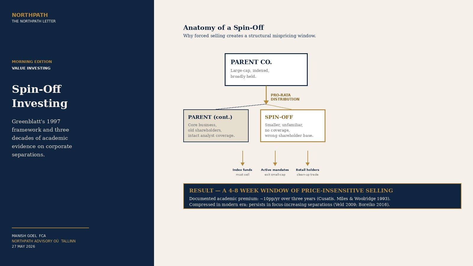
Greenblatt’s argument, stripped to its load‑bearing claims, was this. First, that the new spun‑off security is, at the moment of distribution, in the wrong hands. The original parent’s shareholder base was assembled to own the parent — for index reasons, for sector reasons, for size reasons, sometimes simply because the parent had been in the portfolio for a long time. The spun‑off subsidiary is, by definition, a different business in a different sector at a different size. A meaningful fraction of the inheriting shareholders are structurally compelled to sell within the first weeks: index funds whose mandate excludes the new security, large‑cap funds that cannot hold the smaller spin, sector funds whose mandate excludes the new industry, retail holders who view the unfamiliar new ticker as a clean‑up trade. Second, that this forced selling is largely price‑insensitive — the selling is driven by mandate, not by valuation, and it lands on a security with a tiny circle of natural buyers, no Wall Street research coverage for at least a quarter, no earnings history as a standalone entity, and a shareholder register that is itself in flux. Third, that the underlying business is, on average, structurally healthier after separation: a sub‑scale subsidiary that had been starved of capital under the conglomerate often emerges with sharper management focus, cleaner economics, equity compensation tied directly to its own performance, and the freedom to make capital‑allocation decisions on its own terms.

Greenblatt’s recommended process was almost embarrassingly simple. Read the SEC Form 10 — the registration statement filed by the spun‑off entity ahead of its first day of independent trading — in full. Look for three signals: insider ownership and incentives that align management with the standalone business, a balance sheet whose debt load is appropriate to the new standalone cash flows rather than weighted with the parent’s legacy, and a business that, on its own, the patient investor would want to own at the price implied by the post‑distribution market value. Wait through the initial forced‑selling window — typically four to eight weeks — and act when the technical pressure has cleared. The discipline trades activity for asymmetric exposure: nothing is bought until the structural mispricing is visible in the tape.

2. The Mechanism — Why the Premium Exists at All

The premium does not exist because investors are foolish. It exists because the rules under which the world’s largest pools of equity capital are managed produce a predictable, recurring window in which a subset of listed securities is mispriced for reasons unrelated to the underlying business. Three structural features explain the mechanism, and all three are still in force three decades after Greenblatt described them.

The first is the architecture of indexed and benchmark‑hugging capital. Globally, more than half of equity assets under management are now either passively indexed or run against a benchmark with low tracking‑error tolerance, per Morningstar industry data through 2024. When a parent in the S&P 500 or MSCI World Large Cap spins off a subsidiary that lands, on its first day, in the small‑cap index, the funds tracking the larger index are mandated to sell — not by judgement, but by rule. Active funds benchmarked to the large‑cap index face the same arithmetic. The selling lands on a security whose natural buyers — small‑cap dedicated funds — are themselves not yet positioned to take it, because most have not yet been notified by their benchmark provider that the new ticker is in their universe.

The second is the absence of sell‑side coverage at the moment of listing. Until separation, the standalone subsidiary was a segment in the parent’s annual report. It had no analyst model of its own, no consensus earnings estimate, no broker target price. Analyst coverage usually takes one to two quarters to assemble. Until it does, the spun‑off security trades on Form‑10 filings and management presentations — both available, both requiring work to read. The bias of most short‑term trading capital is to wait for coverage to begin; the result is a window in which the price reflects the marginal seller far more than the marginal informed buyer.

The third — and the one Greenblatt emphasised most — is the change in management incentives at the moment of independence. Inside a conglomerate, the manager of a sub‑scale division is paid against the parent’s consolidated metrics. Capital is rationed by the corporate office. After separation, the same manager runs a public company. Equity compensation is tied to the standalone share price. Capital can be redeployed without permission from a corporate parent. The same business, with the same assets and the same people, can produce materially different financial results in its first three years of independence — not because it has changed, but because the constraints under which it was being run have changed.

3. The Empirical Record — Three Decades of Academic Replication

The interesting thing about Greenblatt’s framework is not that he made the claim. The interesting thing is that the academic literature has, with considerable consistency, replicated it across three decades, three continents, and several methodologies. The exact magnitudes differ, the windows differ, and the statistical significance varies by sub‑sample; but the direction is the same.

The first major academic study was Cusatis, Miles and Woolridge, published in the Journal of Financial Economics in 1993 under the title “Restructuring through Spinoffs: The Stock Market Evidence”. Examining a sample of 161 spin‑offs from US parents between 1965 and 1988, the authors documented a buy‑and‑hold abnormal return of roughly twenty‑five per cent over the three years following the distribution, with the bulk of the excess concentrated in the second and third years rather than the first. Desai and Jain, writing in the Journal of Financial Economics in 1999, extended the sample to 144 spin‑offs through 1995 and identified an important sub‑sample: “focus‑increasing” spin‑offs — those in which the spun‑off business operated in a different two‑digit SIC code from the parent — earned abnormal returns of roughly thirty‑three per cent over the three‑year window, while “non‑focus‑increasing” spin‑offs delivered no statistically significant excess return.

McConnell and Ovtchinnikov, writing in the Journal of Investment Management in 2004, addressed the most pointed critique of the earlier literature: that the excess returns were a small‑sample artefact driven by a handful of outliers. They tested 311 spin‑offs from 1965 to 2000 and showed that the result survived the removal of the largest outliers; the median spin‑off, not just the mean, outperformed the market. Veld and Veld‑Merkoulova published a meta‑analysis in the International Review of Financial Analysis in 2009, pooling 26 studies across the US, the UK, and continental Europe. They concluded that the average announcement‑date return to the parent of 3.0 per cent, and the post‑separation three‑year abnormal return to the spin of roughly 9.6 per cent annualised, were robust to geography and to time period.

Two important caveats appear in the more recent literature. The first, documented by Boreiko and Murgia in the European Financial Management Journal in 2016 for European spin‑offs between 1989 and 2013, is that the magnitude of the spin‑off premium has compressed in recent decades. The 1965‑1988 sample on which Greenblatt’s original number rests included a great many cases in which a conglomerate that traded at a meaningful discount to its sum‑of‑the‑parts handed shareholders a corrected valuation simply by separating. As conglomerate discounts narrowed in the late 1990s and as activist investors began pre‑empting many of the most obvious value‑unlocking transactions, the premium available to the patient generalist after a spin‑off compressed. The second caveat, documented by Chemmanur and Yan in the Journal of Financial Economics in 2004, is that the premium concentrates in spin‑offs that are focus‑increasing — separations that meaningfully change the strategic geography of both the parent and the child. Spin‑offs that are essentially financial engineering, in which the same management team and the same capital‑allocation philosophy continue to run both halves, have not, on average, delivered excess returns.

The honest reading of the literature is therefore this. The spin‑off premium is real; it is global; it is persistent over a thirty‑year window. But it has compressed in magnitude, it concentrates in focus‑increasing transactions, and it requires that the practitioner read the Form 10, separate the genuinely independent spins from the cosmetic ones, and pay attention to insider incentives and balance‑sheet structure. The single number — “ten per cent per year for three years” — was always a textbook average; the practitioner’s number is whatever the practitioner’s discipline can earn within that distribution.

4. Two Historical Episodes

Two episodes, separated by a quarter‑century and an ocean, illustrate the framework in action. Neither is offered as a recommendation; both are case‑studies in why the mechanism works and where it can fail.

The first is the Marriott separation of October 1993. Marriott Corporation split itself into Host Marriott Corporation, which retained the hotel real estate and the historical long‑dated debt, and Marriott International, which retained the asset‑light hotel management and franchising business. The transaction was controversial when announced — Host Marriott carried roughly $2.9 billion of the parent’s senior debt while owning the cyclical real estate; bondholders sued; institutional shareholders who had bought a hospitality compounder found themselves holding a leveraged real‑estate vehicle they had not asked for. In the months following distribution, Host Marriott traded at a substantial discount to its underlying property value, while Marriott International traded close to a fee‑based comparable multiple. Over the subsequent five years, as the US hotel cycle recovered and the debt schedule worked through, the combined value of the two securities materially exceeded that of the pre‑split parent. The episode became the case‑study by which a generation of US analysts learned to read Form 10 carefully and to separate noisy first‑months trading from underlying business value.

The second is the Mercedes‑Benz Group separation from Daimler Truck Holding AG in December 2021. After more than two decades during which Daimler AG had operated as a single listed entity combining the Mercedes‑Benz passenger car franchise with the Daimler Truck business, the European board concluded that the strategic geographies of the two businesses had diverged sufficiently — battery‑electric passenger vehicles on one side, heavy commercial vehicle electrification and hydrogen on the other — to warrant separation. Daimler Truck Holding AG listed on the Frankfurt Stock Exchange on 10 December 2021; the parent renamed itself Mercedes‑Benz Group AG on 1 February 2022. The forced‑selling pattern was textbook: a number of European large‑cap mandates could not hold Daimler Truck; the new entity began trading without the analyst coverage that had attached to Daimler AG for decades; insider equity grants at Daimler Truck were re‑based to the standalone share price. In the first six weeks of independent trading, the two securities together traded at a discount to the implied pre‑separation value; by mid‑2022, as European institutional capital re‑allocated and as analyst coverage of both standalone entities matured, the discount had narrowed. The episode reads as a European replication of the mechanism Cusatis, Miles and Woolridge had documented in the US three decades earlier.

5. The Application Framework — Three Process Disciplines

What follows is not motivational. It is process. The framework is operationally simple and analytically demanding; the simplicity is exactly what makes it survive the cycle.

Discipline one: build a written watch‑list, refreshed quarterly, of announced and pending spin‑offs in the markets in which the investor is willing to commit capital. The pipeline is finite — globally, between 50 and 100 spin‑offs of meaningful size complete each year, with the largest concentrations in the US and Europe. Anchor the watch‑list to the announcement of the corporate separation, not to the distribution date; the announcement is publicly knowable, often six to twelve months before the actual distribution, and provides the analyst with the runway to read the Form 10 (or its UK / European equivalent) once it is filed. The watch‑list is not a buy list. It is a research queue.

Discipline two: read the Form 10 in full, and write a one‑page memo to oneself before any decision. The memo answers three questions: whether the standalone business is one the long‑term investor would want to own at any price; whether the balance sheet handed to the spin is appropriate to its standalone cash flows or saddled with disproportionate parent legacy debt; and whether the equity compensation of the standalone management team is aligned with the standalone business’s long‑term performance. If any of the three questions returns a negative answer, the spin is not actionable for the patient investor regardless of how attractive the first‑day price action looks. The memo is the discipline that separates a framework from a tip.

Discipline three: wait through the technical‑selling window before sizing a position, and size it within a portfolio context. The forced‑selling pattern typically clears within four to eight weeks of distribution. First‑week price action reflects index rebalancing rather than considered valuation; positions established into that window are frequently marked down before the technical pressure clears. The patient investor sizes the position only after the structural sellers have completed their work, and sizes it as a fractional holding within the broader portfolio rather than as a concentrated bet. Spin‑off investing rewards the practitioner who treats each separation as one observation in a portfolio of observations, not as a thesis to be defended.

6. How Long‑Term Practitioners Have Applied It

Greenblatt himself remains the most documented practitioner of the framework. The Gotham Funds, which he co‑founded with Robert Goldstein, ran an explicit spin‑off strategy through the 1990s and into the 2000s; the firm’s reported audited returns from inception of the original Gotham Capital partnership in 1985 through its 1995 closure averaged approximately 50 per cent gross annualised, a figure that Greenblatt has discussed publicly and is documented in his subsequent writing including The Little Book That Beats the Market (2005). The strategy was concentrated, opportunistic, and explicitly tied to corporate events including spin‑offs, recapitalisations, and rights offerings. Greenblatt has been consistent in both the books and the interviews he has given over thirty years that the spin‑off premium is structural, not stylistic, and that the discipline of reading the Form 10 is what converts the structural opportunity into realised return.

A second well‑documented practitioner is Murray Stahl of Horizon Kinetics, whose firm has managed long‑duration equity capital since 1994. In the firm’s quarterly commentaries across the 2010s, Stahl developed the thesis that the academic spin‑off premium concentrates in what he termed “owner‑manager spin‑offs” — separations in which the new standalone entity emerges with strongly aligned insider ownership — and effectively disappears outside that sub‑sample. His framework refines Greenblatt’s by asking the practitioner to focus the research budget on spins in which the people running the new business have a meaningful personal stake in its long‑term success, rather than on the full distribution of separations, most of which are organisational rearrangements with limited insider re‑alignment.

The author of this letter holds no position in any spin‑off or post‑spin entity discussed above.

7. Key Takeaways

First, the spin‑off premium is real and globally persistent over a thirty‑year academic record. It is not an anomaly defying market efficiency; it is a structural consequence of how indexed and benchmark‑hugging capital is mandated to behave in the weeks following a corporate separation.

Second, the magnitude of the premium has compressed since Greenblatt’s 1997 publication, and it now concentrates in focus‑increasing separations in which the parent and the child operate in materially different strategic geographies. Cosmetic spin‑offs and financial‑engineering separations have not, on average, delivered excess returns.

Third, the framework is operationally simple: build a watch‑list, read the Form 10, write a memo, wait through the forced‑selling window. The simplicity is exactly what makes it executable by a generalist long‑term investor without specialised infrastructure.

Fourth, the framework rewards discipline over activity. The pipeline is finite, the actionable subset is smaller still, and the patient investor will commit capital to a small number of separations a year. Treated as one process among several in a long‑term equity portfolio, it is one of the few corners of the market in which structural mispricing is documented, replicated, and still available to the practitioner willing to read the filings.

Fifth, and perhaps most importantly, what Greenblatt’s 1997 chapter actually teaches is a habit of mind that extends well beyond spin‑offs. The habit is to ask, of any apparent mispricing in listed equity, whether there is a structural reason why a particular pool of capital is constrained from acting on what would otherwise be a profitable trade. Wherever mandate, benchmark, or coverage produces forced behaviour at known dates, the patient investor who is not so constrained holds an asymmetric option to act. Spin‑offs are one such corner. There are others. The framework belongs to anyone willing to think about the equity market as a system of constraints as much as a system of prices.

— Manish Goel, FCA / NorthPath Advisory OÜ / Tallinn, Estonia

Important. All content on this site and in this email is journalism and education for a general audience. Nothing here constitutes investment advice or a recommendation in respect of any specific financial instrument, nor an offer or solicitation to buy or sell any security. Readers should consult an authorised financial adviser regulated in their own jurisdiction before making any investment decision.

The NorthPath Letter · Value Investing · Morning Edition · 26 May 2026

Every quoted stock is a sentence the market is whispering to you, in a language most investors never bother to translate. The number on the ticker is not an answer. It is a forecast — a discounted stream of expected future cash flows that the marginal buyer and seller have, between them, agreed to. The disciplined long-term equity investor’s first task is not to build their own forecast and argue with the price, but to read the price as a forecast, decompose it into its operating assumptions, and ask one quiet question: are those assumptions achievable, conservative, or heroic? That inversion of the conventional analytical reflex — start from price, work backward to operating drivers, then test — is the heart of the framework Alfred Rappaport and Michael Mauboussin set out in their 2001 book Expectations Investing. Twenty-five years on, in a market saturated with macro narrative and quarter-by-quarter melodrama, the framework has lost none of its discipline and very little of its edge.

1. The principle: read the price, then test it

Most equity research, even today, follows a familiar choreography. The analyst projects revenue, margins, and capital intensity over a five- to ten-year horizon, discounts the resulting free cash flows to a present value at a chosen weighted average cost of capital, compares that value with the prevailing market price, and renders a verdict. Buy if intrinsic value exceeds price; sell or avoid otherwise. The procedure has the comforting appearance of rigour. In practice, it is almost always defeated by the single weakness it cannot acknowledge: the forecast that anchors it is the analyst’s, and the analyst has no demonstrable edge in forecasting.

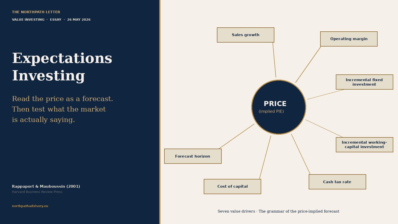
Rappaport and Mauboussin’s framework reverses every step. The market price is taken as given, not contested. The analytical work is to derive — by algebra — the specific combination of sales growth, operating margin, incremental investment rate, tax rate, cost of capital, and forecast horizon that would justify that price exactly. This combination is called the price-implied expectations, or PIE.

The investor’s edge, on this view, comes from being a better judge of whether the PIE is realistic than the marginal market participant. The work shifts from forecasting (a skill in which most investors have no demonstrable edge) to forensic interrogation of consensus assumptions (where a patient, primary-source investigator can develop one). Rappaport and Mauboussin trace the intellectual lineage of this idea to Alfred Rappaport’s earlier work on shareholder value (Rappaport, Creating Shareholder Value, 1986), which articulated the seven value drivers that any discounted cash-flow model rests on. The 2001 book made those drivers the language in which the implied forecast is decoded. The 2021 revised edition, published by Columbia Business School Publishing, updated the worked examples for the post-2008 environment of compressed discount rates and intangible-heavy balance sheets without altering the procedural spine.

2. The mechanism: why surprises, not levels, drive returns

The empirical regularity that gives expectations investing its purchase is straightforward. Over short and intermediate horizons, a stock’s return is dominated not by how the company performs in absolute terms, but by how its performance compares with what was already priced in.

A business growing revenues at twelve per cent a year is a good business. If the market had been pricing in fifteen per cent, the stock will fall on a quarter that delivers twelve. A business growing at six per cent is a mediocre business. If the market had been pricing in three, the stock will rise on a quarter that delivers six. The level of performance is not the operative variable. The change in expectations is.

This is why Mauboussin, in a series of papers written first at Credit Suisse and later at Counterpoint Global, returns again and again to a single metric — what he calls the expectations infrastructure: the small set of operating drivers (volume, price, mix, operating leverage, returns on incremental capital) that explain almost all of the change in market-implied free cash flow. If those drivers move favourably relative to expectations, the stock works. If they move unfavourably, even good absolute performance is insufficient. The pattern holds across geographies and across decades. Studies of US, European, Japanese and emerging-market equity returns since the 1980s consistently show that earnings surprises explain more of the cross-sectional variation in twelve-month forward returns than do absolute earnings growth rates.

For the long-term equity investor, the implication is liberating rather than constraining. Most short-term noise is the marginal participant repricing their expectations on a single quarter of news. The investor who has already done the work of decomposing the PIE and forming an independent view of where each driver will land over five to ten years is not buffeted by that repricing. They are, in many cases, on the other side of it.

3. The empirical record: anchoring, drift, and the inadequacy of multiples

The case for expectations investing rests on three documented regularities, each of which has been replicated in the academic literature across multiple decades and multiple markets.

The first is anchoring. Lichtenstein, Slovic, Fischhoff and Phillips, in their 1982 review in Kahneman, Slovic and Tversky’s Judgment under Uncertainty, showed that human forecasters anchor on the most salient prior estimate. In equity markets, that prior is almost always last quarter’s reported number or consensus estimate. Analyst forecasts cluster within narrow bands around prior outcomes (Easterwood and Nutt, 1999; Cen, Hilary and Wei, 2013). The marginal market participant is, statistically, the analyst — and the analyst is anchored. A disciplined PIE decomposition gives the investor a chance to spot expectations that the consensus has accepted simply because they sit close to the recent past.

The second is post-earnings-announcement drift, first documented by Ball and Brown in 1968, replicated across five decades and almost every major market, and surveyed comprehensively by Bernard and Thomas (1989). Stocks that surprise consensus to the upside continue drifting upward for sixty trading days; stocks that surprise to the downside continue drifting downward. The mechanism is the slow updating of expectations: the marginal market participant takes weeks, not minutes, to reformulate their model. The disciplined PIE investor, who already holds a more accurate view of operating drivers, can position before the drift compounds.

The third is the documented inadequacy of price-to-earnings multiples as a stand-alone valuation tool. A trailing P/E of twelve can be cheap (if the company is in a stable industry with twelve per cent return on incremental capital and no growth) or expensive (if the company faces structural decline). A P/E of forty can be expensive (if growth is decelerating) or cheap (if growth is accelerating and incremental returns on capital are high). Mauboussin’s 2014 Credit Suisse note What Does a Price-Earnings Multiple Mean? demonstrates algebraically that the P/E ratio is itself a compressed statement of price-implied expectations — and that comparing P/Es across companies without unpacking those expectations is meaningless. Expectations investing forces the investor to do the unpacking explicitly.

To these three regularities one might add a fourth, drawn from the Bessembinder long-tail literature that has now been replicated through 2023: a small minority of stocks account for nearly all aggregate equity wealth creation, and those stocks are characteristically ones where the price-implied expectations at the start of the holding period were materially below the realised trajectory. Expectations investing is the procedural counterpart of the long-tail empirical fact: it is the method by which an investor positions for the asymmetric outcome rather than the average one.

4. Two historical episodes where the principle was visible

The Cisco Systems episode of March 2000 is the textbook illustration. At the peak, Cisco traded at a market capitalisation of approximately five hundred and fifty billion United States dollars, with consensus implying revenue growth of more than thirty per cent annually compounded for the following decade. A PIE decomposition by an analyst willing to do the arithmetic would have shown that, even granting generous operating margins, Cisco would need to be capturing essentially all of the global enterprise networking spend by 2010 to justify the price. The required share-of-spend was not achievable; the price was, in the Rappaport-Mauboussin sense, pricing a heroic outcome. Over the following two and a half years, the stock fell by approximately eighty-eight per cent, even as the business itself continued to grow revenue and protect margin. The fall was not a business failure. It was an expectations realignment — and a realignment that was visible in the arithmetic at the peak, to anyone willing to look.

The opposing example is Amazon in late 2001 and through 2002. At points during the post-dot-com winter, Amazon’s market capitalisation implied that operating margins would never expand above one or two per cent, that revenue growth would taper to single digits within five years, and that the company’s investment in fulfilment infrastructure would never earn an adequate return. A PIE decomposition done in 2002 — using Rappaport and Mauboussin’s framework explicitly — would have revealed that the marginal investor was extrapolating short-term losses into permanent unprofitability. Bill Miller, then managing Legg Mason Value Trust and a notable practitioner of expectations-investing language, built a position on exactly that logic. The five-year return on that position exceeded six hundred per cent — not because the business surprised on an absolute basis, but because operating margins and capital efficiency surprised relative to the bombed-out implied trajectory.

A third compact illustration, drawn from the European market, is the Anheuser-Busch InBev sequence from 2018 to 2020, when the brewer’s price implied permanent revenue stagnation and balance-sheet stress; subsequent margin recovery and methodical deleveraging surprised that implied trajectory positively, and the stock recovered roughly seventy per cent from its 2020 lows over the following twenty-four months. The same arithmetic, applied across continents and decades, identifies the same kind of opportunity: a price that has compressed expectations below what the operating reality can deliver.

5. The application framework: three concrete disciplines

The temptation, when introduced to expectations investing, is to treat it as a mental attitude — a sensibility, a way of thinking. It is, in fact, a procedural discipline that can be written down and followed by anyone willing to maintain a working spreadsheet and a primary-source library.

First, decompose the price into a PIE. The investor begins with the market capitalisation plus net debt — enterprise value. From this, they subtract the present value of the next several years of consensus or analyst-built free cash flow forecasts, then solve algebraically for the residual: the long-term growth rate, the terminal margin, or the value-growth duration that would close the gap. Practical implementations require a discounted cash flow spreadsheet with the seven Rappaport drivers (sales growth, operating margin, incremental fixed investment rate, incremental working-capital investment rate, cash tax rate, weighted average cost of capital, and competitive-advantage period or forecast horizon) as adjustable inputs. The investor varies one driver at a time, holding the others at base-case values, and notes the level at which the price is exactly justified. The output is a small table: “the price assumes ten per cent sales growth for fifteen years, OR twelve per cent operating margin in steady state, OR forty per cent return on incremental capital.” Three sentences, derived from arithmetic, that pin down what the market is actually saying.

Second, test each PIE assumption against the operating evidence. This is where Fisher-style scuttlebutt, regulatory filings, capital-cycle data, and primary-source competitor analysis re-enter. If the PIE requires fifteen years of fifteen per cent sales growth, the investor asks: what is the addressable industry growth rate, what share would the company need to gain, what is the historical maximum share for any single competitor in this category, and what would have to be true at the customer or product level for that share-gain to materialise? If the PIE requires twelve per cent operating margins permanently, the investor compares against the highest margin ever achieved in the industry, the margin trajectory of comparable businesses across cycles, and the structural reasons margins might be defensible against the entry of new capacity. The discipline is not to forecast better. It is to test whether the consensus forecast embedded in the price is achievable, conservative, or aggressive.

Third, identify the catalysts that would cause the PIE to revise. Stocks rerate when one or more of the seven value drivers moves materially relative to expectations. The disciplined investor pre-specifies which observable events — a regulatory approval, a competitor exit, a price move, a capital-cycle inflection, a balance-sheet repair — would cause each driver to revise upward or downward, and in roughly what magnitude. They then monitor those specific events rather than the daily price. Position sizing follows from how asymmetric the catalyst set is: if the realistic distribution of revised PIE outcomes is heavily skewed upward, the position is sized larger; if symmetric or skewed downward, smaller or not taken at all.

These three disciplines — decompose, test, monitor — turn a vague philosophical preference for “the market is wrong” into a procedure that can be applied consistently across hundreds of names over decades. That repeatability is what separates a framework from an opinion, and it is what allows the practitioner to keep working through periods of personal doubt and market turbulence without abandoning the method.

6. How long-term-equity practitioners actually applied it

Bill Miller, while running Legg Mason Value Trust between 1991 and 2005, beat the S&P 500 for fifteen consecutive years — a record without precedent in publicly tracked mutual fund history, and one that has not been equalled since. Miller’s process, as documented in Janet Lowe’s The Man Who Beats the S&P (2002) and in Miller’s own quarterly letters, was an explicit application of expectations investing. Miller would identify stocks where, by his arithmetic, the price-implied expectations were materially lower than the realistic trajectory, and hold them through the painful repricing window that follows the catalyst. His Amazon position, his AOL position, and his Dell position in the early 1990s were all built on PIE decomposition rather than absolute-valuation work. Miller wrote and spoke about Mauboussin’s and Rappaport’s framework explicitly through the 1990s and 2000s, often citing the 2001 book by name.

Howard Marks, in his memo “Risk” of January 2006 and in his book The Most Important Thing (2011), discusses the same arithmetic in different language. Marks emphasises that an investor’s return is determined not by what they buy but by what they pay relative to what was expected — and that the price embeds the expectations. Marks’s preference for second-level thinking is, structurally, expectations investing: ask not what the company will do, but what the company will do versus what the market thinks it will do. Marks has returned to this point in memos across two decades, including his 2018 piece on the limits of macro forecasting, and his 2022 memo on the sea change in interest rates, where he framed the rate environment itself as a shift in the implied discount rate baked into every equity price.

Warren Buffett, in the 1992 Berkshire Hathaway letter, sets out what is in substance an expectations decomposition. Discussing the question of whether a stock is dear or cheap, Buffett writes that the only honest test is to compute the discount rate that, applied to the stream of cash the business will produce over its life, equates the present value of those cash flows to today’s price. That discount rate is the rate of return the market price implies. If the investor believes the cash flows will be higher or arrive sooner than the market is pricing, the implied return overstates the achievable return; if lower or later, it understates. The investor’s task is the comparison.

Michael Mauboussin, in his Counterpoint Global notes since 2020, has continued to argue that expectations investing is the only framework that survives contact with empirical asset-pricing data. His 2014 note What Does a Price-Earnings Multiple Mean? decomposes the P/E into its expectations components and shows that almost all the cross-sectional variation in P/E across firms is explained by differences in implied growth and incremental returns on capital, not by differences in “quality” or “story” in any vaguer sense. His more recent work on intangible-heavy businesses applies the same arithmetic to the question of how to capitalise research, development and customer-acquisition expenditure when reading the price of a software or platform business.

These four practitioners — Miller, Marks, Buffett, Mauboussin — converge on the same procedural insight from very different starting points. The convergence is what gives the framework its weight. Each of them, in different vocabularies, is doing the same thing: refusing to argue with the price until they have first decoded what the price is saying.

7. Key Takeaways

The market price of a quoted equity is an embedded forecast, and the long-term investor’s first task is to translate it into specific operating assumptions before having an opinion on whether the stock is dear or cheap.

Stocks rerate on changes in expectations, not on absolute performance levels; the investor who has already decomposed the price-implied expectations is structurally positioned to be on the right side of those changes.

Decomposing a price requires arithmetic, not insight: a discounted cash flow model with the seven Rappaport value drivers, varied one at a time, will reveal what the market is actually saying. The insight comes in the next step — testing those assumptions against the operating evidence.

The discipline replaces forecasting (where most investors have no edge) with the forensic interrogation of consensus (where a patient primary-source investor can develop one); this is the only edge that compounds reliably over decades.

Expectations investing is not contrarian by temperament. It is contrarian by accident, when the arithmetic happens to disagree with the marginal market participant. The investor’s loyalty is to the arithmetic, not to the contrarian posture — and over time, that loyalty is what produces the asymmetry of outcomes the Bessembinder long-tail data so vividly describe.

— Manish Goel, FCA / NorthPath Advisory OÜ / Tallinn, Estonia

Important. All content on this site and in this email is journalism and education for a general audience. Nothing here constitutes investment advice or a recommendation in respect of any specific financial instrument, nor an offer or solicitation to buy or sell any security. Readers should consult an authorised financial adviser regulated in their own jurisdiction before making any investment decision.

VALUE INVESTING  ·  25 MAY 2026  ·  ISSUE 6

The most expensive sentence in long-term equity investing is the one no spreadsheet ever models: most stocks lose money, and a small handful build essentially all the wealth. The intuition that “the market goes up” — the cheerful arithmetic behind every retirement projection ever drafted in a bank branch — is true only as an aggregate of an extremely asymmetric distribution. Pull the average apart and what you find is a long tail of failure, a wide middle of indifference, and a tiny right edge of compounding so extreme that it carries the entire history of equity returns on its back.

Hendrik Bessembinder, a finance professor at Arizona State University’s W. P. Carey School, did the arithmetic that other people had assumed without checking. His 2018 paper, Do Stocks Outperform Treasury Bills? in the Journal of Financial Economics, took every common stock that ever traded on a U.S. exchange between July 1926 and December 2016 and tracked the lifetime dollar wealth each one created above a one-month Treasury-bill benchmark. The result reorganised the way a careful long-term investor should think about diversification, concentration, holding periods, and the value of patience. His 2023 follow-up, co-authored with Te-Feng Chen, Goeun Choi and K. C. John Wei in the Financial Analysts Journal, repeated the exercise across 64,000 stocks in 42 countries between 1990 and 2020. The pattern held everywhere it was measured.

This letter is not a meditation on power laws. It is a working framework for what these two papers should do to the discipline of an investor whose horizon is measured in decades rather than quarters.

1. The Principle

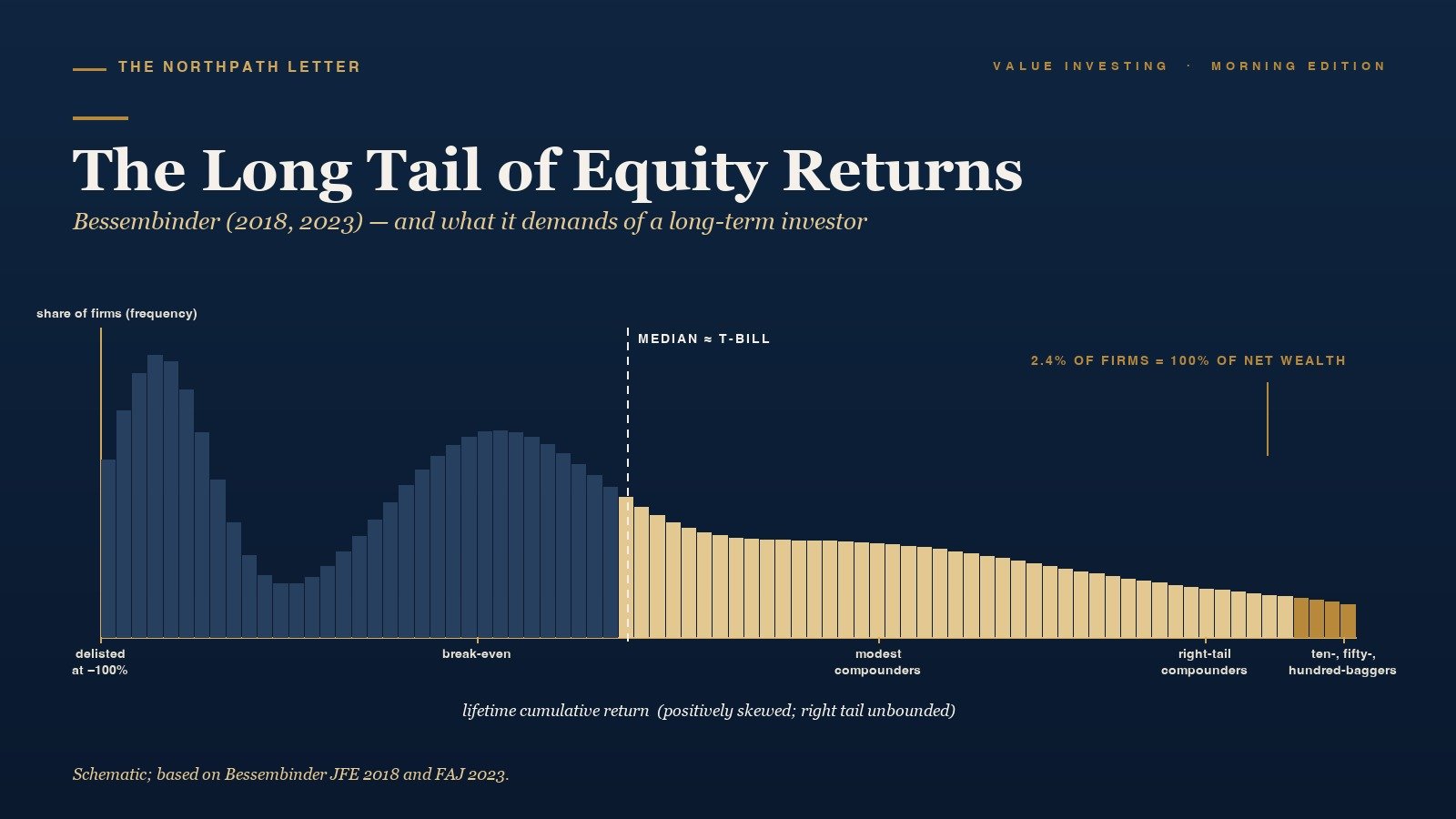
Bessembinder’s principle, reduced to one sentence, is this: the cross-sectional distribution of long-horizon stock returns is so positively skewed that aggregate equity market wealth creation is concentrated in a vanishingly small fraction of firms. The median listed stock, held from listing to delisting, has underperformed a riskless short-dated government bill. The mean stock has comfortably beaten the bill, but only because a tiny right tail of extraordinary compounders has dragged the average upward.

The principle is older than the paper. Maurice Kendall noticed the asymmetry of stock returns in 1953. Eugene Fama wrote about it in 1965. Yakov Amihud, Haim Mendelson, Henrik Hendriksson and Robert Merton, and later Michael Mauboussin in his Counterpoint Global notes, have all returned to it. What Bessembinder did was take the question out of the realm of statistical theory and into the realm of dollars. He counted the wealth.

The translation for a practitioner is uncomfortable. If most stocks lose, then “buy and hold a basket” is not a strategy by itself — the basket matters profoundly. If a few firms built all the wealth, then missing them is not a small cost — it is the cost. And if those firms compounded over multi-decade windows, then the investor’s principal edge is not insight into next quarter’s print but the willingness to remain invested in the right names for far longer than the consensus thinks is reasonable.

2. The Mechanism — Why the Distribution Is Asymmetric

Three structural features of equity ownership produce the long-tailed shape Bessembinder measured.

The first is asymmetric payoff geometry. An equity’s downside is bounded at minus one hundred percent. Its upside is unbounded — a stock that returns one hundred times its purchase price in twenty years is a real outcome that has occurred many thousands of times in market history. When some outcomes are capped at minus one and others are uncapped on the upside, the distribution of compounded outcomes cannot be symmetric. Even if the central tendency of returns were perfectly normal, compounding alone would generate a positively skewed cross-section.

The second is survivorship and self-selection in firm life cycles. Most listed companies do not survive thirty years. They are acquired, delisted, bankrupted, or liquidated. The few that survive long enough to compound for three or four decades are a heavily filtered subset — the survivors are not random. Companies that endure tend to share characteristics (capital-light franchise economics, durable customer demand, disciplined capital allocation, reinvestment opportunities at high incremental returns) that themselves predict further compounding. Survival and compounding feed each other.

The third is winner-take-most economics in product markets. In industry after industry, network effects, scale economics in distribution, and the option value of reinvestment have produced a small number of dominant firms that capture an outsized share of industry profits. The “long tail” in stock returns is, in part, a reflection of the “long tail” in product-market economics. The same handful of firms — Apple, Microsoft, Amazon, Alphabet, Tencent, Samsung Electronics, Taiwan Semiconductor, Nestlé, Roche, LVMH — that dominate the wealth-creation league tables are the same firms whose product-market positions allowed them to reinvest decade after decade at high returns on incremental capital.

The investor’s discipline must be built to fit the shape of the distribution it operates inside. A normal-distribution mindset — “I will own forty stocks, hold them for two years, harvest the average” — collides with the geometry. It is precisely because a few stocks build all the wealth that owning the wrong few is so expensive, and selling the right ones early is the most common form of capital destruction long-term investors inflict on themselves.

3. The Empirical Record

The numbers from Bessembinder (2018) are worth committing to memory because they reframe so many practitioner debates at once.

Of the 25,332 common stocks that traded on U.S. exchanges between July 1926 and December 2016, only 42.6 percent generated a lifetime buy-and-hold return that beat holding one-month Treasury bills over the same window. The median stock returned a lifetime cumulative -3.7 percent and was listed for only seven and a half years before being delisted, acquired, or going bankrupt. Of the same universe, 1,092 firms — about 4.3 percent of the total — accounted for all of the roughly $35 trillion of net wealth that listed U.S. equities created above the riskless rate. The other 24,240 stocks collectively contributed zero. The top 86 firms alone (just over one-third of one percent of the universe) generated half of that $35 trillion. The single largest wealth creator over those ninety years was ExxonMobil, followed by Apple, Microsoft, General Electric, IBM, Altria, Walmart, AT&T, Procter & Gamble and Chevron — the names a sceptical investor of 1990 would have called “boring” right up to the moment they realised what compounding could do.

Five years later, Bessembinder, Chen, Choi and Wei (2023) repeated the exercise across 64,394 common stocks in 42 non-U.S. countries plus the U.S. between January 1990 and December 2020. The pattern was not American — it was structural. Across the entire 31-year global sample, 55.2 percent of non-U.S. stocks delivered negative compound returns. Just 2.4 percent of firms accounted for the entire net dollar wealth creation above the one-month U.S. T-bill of roughly $75.7 trillion. The five top global wealth creators were Apple, Microsoft, Amazon, Alphabet, and Tencent. The top non-U.S. names included Samsung Electronics, Taiwan Semiconductor Manufacturing, Tencent, Nestlé, Roche, Novartis, Toyota, LVMH, HSBC, Royal Dutch Shell and AstraZeneca. Concentration of wealth creation in a thin right tail was not a feature of one country, one era, or one regulatory regime. It was a feature of the asset class.

These are not academic curiosities. They are the empirical floor on which the rest of the practitioner conversation about diversification, concentration, and holding periods has to sit.

A particularly underappreciated finding sits inside the 2023 paper. When the authors compute the proportion of net wealth that came from firms outside the United States, the figure for the 1990-2020 window is roughly 42 percent — over $31 trillion of net wealth above U.S. T-bills was created outside the U.S. equity market. The right tail is not an American export. The non-U.S. portion of the right tail is also more concentrated within each country than the U.S. portion is — in Korea a handful of chaebol and Samsung Electronics dominate; in Taiwan, TSMC alone carries an enormous fraction of the country’s wealth creation; in Switzerland, Nestlé, Roche and Novartis between them account for the majority of national equity wealth. Country-level concentration of the right tail is a real, repeated, and structural feature of the global cross-section.

4. Two Historical Episodes

The first episode is Japan, 1990 to 2024. The Nikkei 225 peaked on 29 December 1989 at 38,915 and did not durably regain that level until early 2024 — a generational drawdown of thirty-four years. To the index-level observer, Japanese equities were a graveyard. To the cross-sectional observer, Japan was a beautifully clean example of Bessembinder’s long tail. Inside that thirty-four-year flatline, Keyence compounded at roughly 19 percent annually in yen terms; Fast Retailing (Uniqlo’s parent) compounded comparably; Nintendo, Shin-Etsu Chemical, Hoya, Daikin, and Sysmex compounded across the same window. The index aggregated zero because the long left tail of bank, real-estate and zombie-industrial stocks offset the right-tail compounders almost exactly. An investor who owned the Nikkei flatlined for a generation; an investor who owned a concentrated set of the right-tail Japanese firms compounded as well as anyone in the world.

The second episode is the pandemic dislocation of 2020 to 2022. Between February 2020 and October 2022 the MSCI All-Country World Index traded sideways in dollar terms — a few percent up, a deep drawdown in 2022, recovery thereafter. The aggregate told one story. The cross-section told another. ASML, Taiwan Semiconductor, Tencent (for the first half of the window), Microsoft, Apple, Amazon, Alphabet, Eli Lilly, LVMH and Hermès compounded heavily through the dislocation; cruise lines, legacy airlines, fossil-fuel-only utilities, and a long roster of legacy retailers and media businesses went sideways or shrank. Once again the index was the algebraic sum of a long left tail and a thin right tail — and an investor’s experience depended entirely on which side of the distribution they had positioned themselves on.

Two episodes, three continents, thirty years apart, the same shape. The long tail is not a U.S. phenomenon, not a tech phenomenon, not a bull-market phenomenon. It is a feature of the asset class, visible in every well-measured window of any reasonable length.

5. The Application Framework — Three Disciplines

The long-tail finding does not licence indiscriminate concentration, and it certainly does not licence the “find the next Apple” speculation that pollutes the popular literature. What it does is reframe three concrete practitioner disciplines.

Discipline one — hold the right tail with both hands. The most common error a long-term investor makes is selling a position that has begun to compound at high incremental returns on capital. Trimming “because it’s gotten too big in the portfolio” is, in Bessembinder’s arithmetic, the precise act of clipping the right tail that builds aggregate wealth. The discipline is not to refuse to ever sell — it is to require an explicit, written, falsifiable thesis for why the underlying franchise economics have deteriorated before reducing a position that the market is willing to reward. Position-size drift caused by compounding is not a problem to be corrected; it is the outcome the strategy was designed to produce.

Discipline two — diversify on the left, concentrate on the right. Bessembinder’s data do not say “own one stock.” They say that the right tail is irreducibly hard to identify ex ante, that the left tail is real and ruinous, and that the rational practitioner therefore wants enough names in the portfolio that any single left-tail outcome does not break compounding, while also being willing to let the right-tail names grow without artificial caps. In practice this often resolves to a portfolio of fifteen to twenty-five carefully chosen long-duration franchises, with the strongest five or six allowed to drift to twenty, thirty, or forty percent of capital over a multi-decade holding period.

Discipline three — extend the holding period until the right tail can express itself. Bessembinder’s wealth-creation calculations are computed over the full listed life of each stock. They cannot be reproduced in a one-year, three-year, or even five-year window. The right tail in his data took a median of two to three decades to fully express itself. An investor whose typical holding period is eighteen months is functionally invisible to the long-tail engine — they are trading inside a window too short for the geometry to matter. Extending the typical holding period from two years to ten years is, in long-tail terms, more important than any improvement in stock-selection accuracy at the front end. This is the principle Michael Mauboussin has elsewhere called “time arbitrage” — the structural edge of a holder who can wait when most market participants cannot.

6. How Practitioners Have Applied It

Three named practitioners have built portfolios whose discipline maps closely onto Bessembinder’s empirical regularity.

Charlie Munger wrote and spoke for fifty years about the same observation, well before Bessembinder formalised it. In his 1995 Harvard speech on the psychology of human misjudgment, and across the annual meetings of Daily Journal and Berkshire from 1995 to 2023, Munger returned again and again to the same theme: the rational long-term portfolio is the one that owns a small number of “wonderful businesses” and holds them across decades. His personal portfolio at death held three names. Berkshire Hathaway’s listed equity book, at its peak post-2010 concentration, had roughly 40 percent of its weight in a single name (Apple) and over 70 percent in its top five positions. Munger’s repeated answer to the question of why he diversified so little was direct: because the right tail is where the compounding lives, and refusing to let it run is what most professional investors do wrong.

Nick Sleep and Qais Zakaria ran the Nomad Investment Partnership from 2001 to 2014 with an explicit doctrine that closely anticipated Bessembinder. In the Nomad letters (collected and published in 2021), Sleep wrote repeatedly about “scale economies shared” — the small set of companies that pass operating leverage back to customers as lower prices and so widen their moat over decades. Nomad’s portfolio at closure in 2014 consisted of three positions: Amazon, Costco, and Berkshire Hathaway. Each had been held for many years; each was deeply researched at the franchise-economics level; each was sized to a level that would have made a conventional risk officer protest. Nomad returned its investors approximately twentyfold over thirteen years before voluntarily winding down. The structure of the result was Bessembinder’s distribution as a portfolio policy.

Tom Russo at Gardner Russo & Quinn has run the Semper Vic Partners and Global Family Branded Equity funds along similar lines since the late 1980s. His top ten holdings have for decades represented roughly two-thirds of the fund’s assets — Nestlé, Heineken, Pernod Ricard, Brown-Forman, Mastercard, Berkshire Hathaway, and a small set of other multi-decade brand franchises. Russo’s central concept, which he calls the “capacity to suffer,” is the discipline of accepting reported-earnings drag from long-cycle reinvestment by management teams who are building thirty-year businesses. The discipline maps directly onto Bessembinder: the firms that built the right tail were almost never the most reported-earnings-efficient firms in any single year. They were the firms whose owners let them reinvest, year after year, at high returns on incremental capital, and stayed in the seat long enough for the geometry to compound.

Three other practitioners are worth naming in passing because their portfolios have been built around the same shape of distribution. Terry Smith at Fundsmith Equity has run a portfolio of roughly twenty-five to thirty long-duration consumer and software franchises since 2010, with the explicit doctrine “do nothing” once the franchises are owned. Chuck Akre at Akre Capital Management built the Akre Focus Fund around a three-legged stool of business quality, capable management, and reinvestment runway — and let the strongest names (Mastercard, Visa, American Tower, Moody’s) compound to thirty and forty percent weightings in the portfolio over more than a decade. Christopher Hohn at TCI Fund Management runs a deeply concentrated long-duration book that has at times held just eight to ten positions. In every case, the portfolio architecture is recognisable as a deliberate attempt to ride the right tail of the distribution rather than to average it away.

7. Key Takeaways

First, the equity return distribution is not normal. It is positively skewed at the security level and the asymmetry strengthens as the holding period lengthens. Aggregate market wealth is built in a thin right tail, in any country and any era so far measured.

Second, the median stock loses to the riskless rate over its listed life. The mean stock wins only because of the right tail. An investor who diversifies broadly without holding the right tail is, in expectation, owning the middle of the distribution — which is where wealth is not created.

Third, the practitioner response is not “buy the index and look away” — that is a structurally sound but emotionally easier path. The active practitioner response is to own a small set of carefully chosen long-duration franchises, accept that the position weights of the right tail will drift upward as the strategy succeeds, and extend the holding period far beyond what conventional turnover statistics imply.

Fourth, identifying the right tail in advance is irreducibly hard. The discipline is therefore to put the weight of the work into franchise quality, capital allocation discipline, and management durability — the structural predictors of the right tail — and to accept that even a careful process will miss most of the future winners. The point is not to own all of them. The point is to own enough of them, large enough, for long enough, that the geometry can do its work.

Fifth, the time horizon is the single most underused free variable in the long-term investor’s toolkit. Bessembinder’s calculations are denominated in lifetimes. An investor whose effective holding period is two years cannot, by construction, harvest a phenomenon that takes two to three decades to express itself. Extending the holding period is not a stylistic preference. It is the precondition for the long-tail engine to operate inside one’s own portfolio.

— Manish Goel, FCA / NorthPath Advisory OÜ / Tallinn, Estonia

Important. All content on this site and in this email is journalism and education for a general audience. Nothing here constitutes investment advice or a recommendation in respect of any specific financial instrument, nor an offer or solicitation to buy or sell any security. Readers should consult an authorised financial adviser regulated in their own jurisdiction before making any investment decision.

VALUE INVESTING · MORNING EDITION · 24 MAY 2026

The single most powerful sentence Warren Buffett has ever written about Berkshire Hathaway is also the shortest. Discussing the firm’s insurance operations in the 2009 shareholder letter, he defined the engine of its multi-decade compounding in nine words: “Float is money we hold but do not own.” Read those words slowly. They are the door behind which the most important structural advantage in modern long-term equity investing has been hiding in plain sight for nearly six decades, and they are the reason why a private investor in 1965 who bought a single share of Berkshire at $19 owned, by 2024, an asset trading above $700,000. The pages that follow examine the principle in the form a serious global long-term equity investor must understand it: not as a piece of Buffett trivia, but as a mental model for recognising where leveraged compounding actually comes from, what discipline it demands of the capital allocator, and which of its features can and cannot be replicated outside the insurance industry.

1. The principle: what float actually is

Float, in the precise insurance-accounting sense Buffett uses, is the difference between what an insurer has collected in premiums and what it will eventually pay out in claims. It is the cash held on the balance sheet against future obligations — technically, the sum of loss reserves, loss-adjustment-expense reserves and unearned premiums, less insurance receivables, deferred acquisition costs and certain prepaid expenses. The definition first appeared informally in Buffett’s 1967 letter, the year after Berkshire acquired Jack Ringwalt’s National Indemnity for $8.6 million. It was made rigorous in the 2009 letter and has been repeated, almost verbatim, in every subsequent annual report.

The crucial property of float is that, although it sits on the asset side of the balance sheet as cash and securities, it does not belong to the insurer. It is held in trust, against claims that will, eventually, be paid. From the perspective of generally accepted accounting principles, float is a liability. From the perspective of the practising investor it is something far more interesting: it is a pool of capital the insurer can invest, for as long as the policies remain in force, without paying interest. If the insurer’s underwriting is disciplined enough that premiums earned exceed expected losses and operating costs, the cost of float drops below zero. The insurer is then being paid by its policyholders for the privilege of investing their money.

This is the source of Buffett’s most-quoted, most-misunderstood claim. He has written, repeatedly, that Berkshire’s float has carried “a negative cost” over the long run. He does not mean that Berkshire has somehow defied the basic arithmetic of insurance. He means precisely that, year after year, premiums have exceeded claims and expenses by enough to add an underwriting profit on top of the investment returns generated by the float pool. The leverage is not borrowed; it is given. That single fact, more than any other, is what separates Berkshire’s compounding record from every other long-only equity vehicle of the last sixty years.

2. The mechanism: three structural advantages compounding at once

A long-term investor analysing float as a principle, rather than as Berkshire trivia, must isolate three distinct mechanical advantages that operate simultaneously. None of the three is exotic. What is exotic is the way the insurance balance sheet bolts them together.

The first advantage is duration. Property-and-casualty policies on average pay out claims years after the premium is collected. Long-tail lines — workers’ compensation, professional liability, medical-malpractice reinsurance, super-catastrophe reinsurance — can stretch a single premium-to-claim cycle to ten or fifteen years. Over that horizon the float behaves, economically, like permanent capital. Berkshire’s reinsurance subsidiary, BHRG, run since 1986 by Ajit Jain, was specifically constructed to maximise this duration advantage, accepting low-frequency, high-severity risks that almost no one else would underwrite on terms that left the underlying float economically permanent.

The second advantage is cost. Conventional corporate leverage costs whatever the bond market charges — today, for an investment-grade industrial, perhaps four to six per cent before tax. Float costs whatever the underwriting loss ratio in excess of one hundred per cent turns out to be, plus or minus operating expenses. For an insurer that prices risk competently, that number is zero. For one that prices risk well, it is negative. Buffett has reported that Berkshire’s float has carried a negative cost in most years since the mid-1990s; the AQR paper Buffett’s Alpha (Frazzini, Kabiller and Pedersen, Financial Analysts Journal, 2018) decomposes Berkshire’s long-run leverage at an average of 1.7 times equity and concludes that the “cheap and stable” nature of that leverage explains a material fraction of the return advantage over the broad market.

The third advantage is non-recourse. A holder of Berkshire debt or equity may, in a crisis, demand repayment, sell the stock, or refuse to roll a maturing bond. A policyholder cannot. The policy obligates Berkshire to pay claims as they emerge, on terms set when the policy was written, in cash that the insurer accumulates over the life of the policy. There is no margin call on float. The 2008 financial crisis is the cleanest demonstration: every leveraged financial company in the United States that depended on overnight funding hit a wall in September 2008. Berkshire’s insurance balance sheet, by contrast, was unaffected. The float pool did not run; the policies did not lapse; the cash continued to come in faster than it went out.

These three mechanical advantages — long duration, near-zero cost, and non-recourse character — combine multiplicatively, not additively. A long-duration pool of capital that pays nothing to use and cannot be withdrawn by its owners is the closest thing to perpetual equity that finance has ever produced. Buffett’s achievement is not that he discovered this; the insurance industry has known about float since the seventeenth century. His achievement is that he reinvested the float, year after year, in operating businesses and listed equities at returns that compounded the entire structure at twice the rate of the underlying market.

3. The empirical record

The numbers are public and, by any standard of modern finance, unprecedented. Berkshire’s float was approximately $19 million in 1967, the year after Buffett bought National Indemnity. It reached $1.6 billion in 1990, $28 billion in 2000, $66 billion in 2010, and $169 billion by year-end 2023. The compound annual growth rate of the float pool over fifty-six years is approximately 17.4 per cent. Over the same period Berkshire’s per-share book value compounded at 19.8 per cent against 9.9 per cent for the S&P 500 total return index. The gap of roughly nine percentage points per annum, sustained over more than half a century, is the largest documented excess return of any long-only equity vehicle in the history of public markets.

The AQR decomposition, published in the Financial Analysts Journal in 2018, attempted to deconstruct that record into systematic factors. The authors found that Berkshire’s portfolio could be substantially explained by a combination of quality, low-beta and value exposures — well-known equity-style factors — but only when the analysis was adjusted for leverage of approximately 1.7 times. The source of that leverage, the paper makes plain, was overwhelmingly insurance float rather than bank debt or capital-markets funding. Stripped of float leverage, Berkshire’s book value would have compounded at perhaps 13 to 14 per cent rather than 19.8 per cent. The float, in other words, did not create the alpha. It magnified, durably and cheaply, an underlying stock-selection process that was already excellent.

For a global long-term equity investor the implication is not motivational. It is structural. The single most powerful documented source of post-war compounding came from coupling competent value-investing judgment with a particular kind of liability structure. Investors who imitate the judgment without understanding the liability structure are imitating only half of what made the record possible.

4. Two historical episodes

Float is easier to see in moments where it nearly broke than in moments where it worked smoothly. Two episodes, on two continents and twenty-five years apart, are instructive.

Berkshire’s acquisition of General Re in 1998 remains the most expensive lesson in the literature about what happens when an investor buys float without underwriting discipline. Berkshire paid approximately $22 billion in stock for General Re. The acquired company brought with it about $15 billion of float — on paper, a transformative addition. In practice, General Re was carrying inadequate reserves on long-tail liability lines, underwriting at combined ratios above one hundred per cent, and exposed to terrorism risk that crystallised disastrously on 11 September 2001. The 2001, 2002 and 2003 letters carry an unusually frank Buffett admission that the float Berkshire had bought turned out to be expensive float for the first four to five years after the acquisition, requiring fresh capital injections to rebuild reserves and a complete rebuild of underwriting culture under new management. Only by approximately 2006 did General Re return to underwriting profitability. The lesson, set down in the 2001 letter and never softened since, is that the value of float depends entirely on the discipline of the underwriting that creates it. Float is not capital that an outsider can simply acquire. It must be earned, year after year, by pricing risk correctly.

Lloyd’s of London 2001-2003 tells the same story in mirror image. The London market, structurally fragmented across hundreds of syndicates underwriting through individual Names, lost approximately $5 billion in 2001 alone. Reserves across the market proved inadequate; several Names were ruined; the corporate-capital reforms that had begun in the mid-1990s were accelerated to recapitalise the market. Crucially, the syndicates that emerged strongest from the cycle — Catlin, Hiscox, Beazley, and the rebuilt Equitas run-off vehicle — were the ones whose 1998 and 1999 underwriting had been most conservative. The investor who bought a Lloyd’s vehicle in 1999 because of the float it generated, without examining the quality of the underwriting that produced it, paid a steep price in 2001 and 2002. The investor who bought after the reserve clean-out in 2003, at trough valuations, into syndicates with demonstrably disciplined underwriting, compounded capital at exceptional rates for the next decade.

The Indian general-insurance industry, opened to private competition by the Insurance Regulatory and Development Authority Act of 1999 and the entry of ICICI Lombard, Bajaj Allianz and HDFC Ergo from 2001 onward, offers a regional variant of the same lesson. Gross general-insurance premiums in India grew from roughly ₹10,000 crore at liberalisation to approximately ₹3 lakh crore by FY24, an order-of-magnitude expansion of the float pool. But Indian insurers operate under IRDAI investment regulations that restrict the proportion of float that may be deployed into listed equities — typically capped between 25 and 30 per cent depending on product class. The structural Berkshire model — deploying float aggressively into operating businesses and concentrated equity positions — is, by regulation, unavailable to any Indian insurer. The Indian listed insurance sector therefore behaves more like a high-quality financial business growing in line with premium volume than like a compounding leveraged equity engine. The structural insight matters: float is not magical in itself. Its productivity depends on what an investor is permitted, by mandate or regulation, to do with it.

5. The application framework: three disciplines

For a global long-term equity investor — one who will not, in practice, ever own and operate an insurance company — the principle of float translates into three disciplines that apply across the broader portfolio.

The first discipline is to recognise float-equivalents in non-insurance businesses. A negative working-capital cycle is structurally identical to float, in miniature. Costco collects cash from members at the till and pays its suppliers thirty days later; the difference is a perpetual interest-free loan from the supplier base that funds inventory. Hindustan Unilever in India has operated with deeply negative working capital for decades, financing growth from trade credit. Bajaj Finance, although technically an NBFC rather than an insurer, generates a comparable structural advantage through deposit-funded lending. The right question for any analysed business is not whether it has float in the literal insurance sense but whether some part of its operating cycle is funded by counter-parties who do not charge for the use of their capital. Where the answer is yes, the business carries a hidden source of leverage that orthodox return-on-equity calculations under-weight.

The second discipline is to refuse, in personal capital, to provide free float to other people’s businesses. A long-term equity investor who buys a subscription product, pays for an annual product in advance, or holds a deposit with a low-yielding institution is, in microcosm, supplying float. This is unobjectionable when the supplier is a household business with whom you have other reasons to deal. It is dangerous when the supplier is a financial intermediary whose business model depends on collecting other people’s capital cheaply. The careful investor inventories, periodically, where their own working-capital float is being given away.

The third discipline is to distinguish, when analysing insurers as investments, between underwriting discipline and float accumulation. Almost every insurer in the world will eventually publish a chart of growing float. Almost none of them will publish a candid analysis of the cost of that float over a full cycle. The investor must do that analysis from the financial statements: a combined ratio averaging above one hundred per cent over a full underwriting cycle, including the bad years, means the float carries a positive cost and the insurer is, in substance, an expensively-funded asset manager. A combined ratio averaging below one hundred per cent means the float is free or negative-cost and the insurer is, in substance, a leveraged compounding vehicle of the Berkshire type. The label on the front of the annual report tells you nothing useful. The combined ratio across the cycle tells you everything.

6. How long-term equity practitioners applied the principle

Three figures in the value-investing lineage have, between them, mapped the practitioner application of float economics over six decades.

Warren Buffett, in the 1967, 1995, 2009 and 2023 Berkshire shareholder letters, is the canonical source. The 1995 letter set out his reasoning for paying $2.3 billion for the half of GEICO that Berkshire did not already own — a deal struck because GEICO’s low-cost direct-marketing model produced disciplined underwriting and a fast-growing float pool that could be redeployed at higher returns inside Berkshire than inside GEICO’s own portfolio constraints. The 2009 letter set out the formal definition of float and traced the firm’s float arithmetic from 1967 forward. The 2023 letter records the figure that has come to define the principle: Berkshire’s float at year-end 2023 stood at $169 billion, supporting investment portfolios valued at multiples of that figure and underwriting that, taken across the prior twenty years, had produced cumulative pre-tax underwriting profit running into the tens of billions of dollars. Disclosure: the author holds no position in Berkshire Hathaway and no position in any of the listed insurers discussed in this essay.

Henry Singleton, the founder of Teledyne, applied a structurally similar idea outside the insurance industry. As William Thorndike documents in The Outsiders (Harvard Business Review Press, 2012), Singleton acquired Argonaut Insurance in 1969 and Unitrin’s precursor businesses through the 1970s, generated cash from those insurance subsidiaries, and used the proceeds — alongside cash flow from Teledyne’s industrial divisions — to retire ninety per cent of Teledyne’s outstanding shares over a twelve-year period. The mechanism is different from Berkshire’s — Singleton used the cash for buybacks rather than for portfolio investment — but the economic substance is the same: an insurance subsidiary supplied long-duration, low-cost capital that an exceptional allocator deployed at compound rates the parent company could not have funded otherwise. Teledyne’s share price compounded at 17.9 per cent annually from 1963 to 1990 against approximately 8 per cent for the S&P 500 over the same window.

Prem Watsa, who founded Fairfax Financial Holdings in 1985 with the explicit intention of building “a Canadian Berkshire,” offers the cleanest test of whether the principle is replicable. Fairfax’s float grew from approximately $20 million in 1985 to over $30 billion by 2023, compounded by acquisitions of Crum & Forster, Northbridge, Zenith National, Allied World and others. Book value per share has compounded at approximately 17 per cent annually since inception, a remarkable record but materially below Berkshire’s. The decomposition of the gap is instructive: Fairfax’s underwriting has been more cyclical than Berkshire’s, particularly through the 2008-2014 macro-hedge programme that crystallised large losses, and Fairfax’s equity-investment record, while strong, has been less concentrated and less consistent than Buffett’s. The model works. It is, however, more demanding of underwriting and investment judgment in equal measure than its apparent simplicity suggests.

What the three records share is the underlying architecture. A pool of long-duration, low-cost, non-recourse capital, supplied by counter-parties who are not in the business of demanding returns on it, can be deployed by a disciplined allocator at rates that compound the entire structure faster than the underlying market for decades on end. The architecture is rare because both halves — the underwriting and the allocation — must be world-class at the same time, in the same firm, for the same multi-decade period. There is no shortcut to either half.

7. Key takeaways

1. Float is the difference between premiums collected and claims yet to be paid. Properly underwritten, it is a pool of long-duration, low-cost, non-recourse capital available for investment for as long as the policies remain in force.

2. Berkshire Hathaway’s 19.8 per cent multi-decade book-value compounding is, on the AQR 2018 decomposition, the product of an excellent underlying value-investing process amplified roughly 1.7 times by cheap and stable float leverage. The leverage did not create the alpha; it magnified it.

3. Float is not a free good. Its value depends entirely on the discipline of the underwriting that creates it. Buying float without underwriting discipline — the General Re lesson of 1998 to 2003 — converts an apparent asset into an expensive liability.

4. The principle generalises beyond insurance. Negative working-capital businesses, deposit-funded lenders, and any operating model funded by counter-parties who do not charge for the use of their capital share part of float’s structural advantage. The careful investor looks for it explicitly in the operating cycle of every business they own.

5. Replicating the full Berkshire architecture requires both world-class underwriting and world-class capital allocation, sustained in the same firm for decades. Three practitioners — Buffett at Berkshire, Singleton at Teledyne, Watsa at Fairfax — have shown it is possible. None of the three has made it look easy.

— Manish Goel, FCA / NorthPath Advisory OÜ / Tallinn, Estonia

Important. All content on this site and in this email is journalism and education for a general audience. Nothing here constitutes investment advice or a recommendation in respect of any specific financial instrument, nor an offer or solicitation to buy or sell any security. Readers should consult an authorised financial adviser regulated in their own jurisdiction before making any investment decision.